TI energy-sweep symbolic reuse + the dense σ(E) cross-section curve
Location: the reuse lives in qscat.linalg.SparseLU.refactor(A_new)
(backed by _ScipyBackend.refactor / _MumpsBackend.refactor in
qscat.linalg._mumps_backend); the wired sweep is in
projects.n2_2d_cross_section.cross_section_2d.ve_cross_section_2d. The
display is the experiment-agnostic
projects.n2_2d_cross_section.cross_section_plot.plot_cross_sections plus the
N₂ driver validation.n2.ti_curve. Benchmark: benchmarks/sweep_reuse.py.
Figure: docs/physics/figures/n2-2d-ti-cross-section.png (+ regenerable
.npz). Origin: sub-project #9; builds directly on #6 (the exact 2-D
driven solver) and #8 (the MUMPS backend, see
docs/physics/mumps-sparse-backend.md). Units: atomic units throughout.
The idea: one symbolic analysis, many numeric factorizations
A driven-equation cross-section sweep factors \(A(E) = E_\mathrm{tot}\mathbb{1} - H\) once per
collision energy and solves against the driving term. Across the sweep only the
scalar diagonal shift E_tot·I changes — H is fixed, and the identity merely
shifts the already-populated diagonal — so every A(E) has an identical
sparsity pattern. A sparse direct solve has two separable phases:
Symbolic analysis — fill-reducing ordering (SCOTCH nested dissection on the MUMPS backend) + symbolic factorization. Depends only on the pattern.
Numeric factorization — the actual
LDLᵀvalues. Depends on the entries.
Because the pattern is E-independent, the analysis is correct for every energy
in the sweep and need be done only once; only the numeric factorization
must repeat. MUMPS exposes exactly this split: factor(reuse_analysis=True)
re-uses the stored analysis on the persistent Context and skips the ordering.
SparseLU.refactor(A_new)
refactor re-runs only the numeric factorization, reusing the symbolic
analysis from construction:
MUMPS backend:
set_matrix(a); factor(reuse_analysis=True)on the sameContext— the SCOTCH ordering is not recomputed. This is where the reuse win materializes.scipy/SuperLU backend: SuperLU has no clean symbolic-reuse hook, so
refactorhonestly re-runssplu(A_new)— correct, but no speedup. SuperLU remains the always-available fallback and the differential oracle.Pattern guard (a correctness requirement, not an optimization):
reuse_analysis=Trueis valid only for an identical nonzero structure — reusing an ordering computed for a different pattern would silently produce a wrong factorization. Each backend stores the analyzed matrix’s canonicalized(indices, indptr)pattern (of the supplied matrix — thetriuupper triangle on the SYM=2 symmetric path, the full matrix otherwise) andrefactorraisesValueErroron any shape or structure mismatch. A diagonal shiftE_tot·I − Halways passes; a genuinely different matrix is rejected.refactorkeeps the same backend and symmetry decision as construction (the analysis assumed them).
The reuse is bit-identical: SparseLU(A0); lu.refactor(A1); lu.solve(b) equals
a fresh SparseLU(A1).solve(b) to round-off. Verified on the MUMPS backend
across several distinct diagonal shifts at real N₂ 2-D scale (rel err ~7e-16,
matching a fresh SuperLU solve), and on the scipy path on the dev box.
The wired sweep
ve_cross_section_2d now sweeps analyze-once/refactor-per-energy. It builds the
solver lazily at the first open (E > 0) energy (SparseLU(A(E)) —
analyze + factor) and refactor(A(E)) for every subsequent open energy;
below-threshold energies (E ≤ 0) return zeros with no factorization at
all (there is no scattering solution below threshold). The returned σ, its
scalar/array shape contract, and the return_wavefunction behavior are
unchanged — the physics is identical, only the factorization path differs.
The per-energy \(E_\mathrm{tot} = E + \varepsilon_{v_\mathrm{init}}\) (the e_tot argument) fed to refactor is exactly the value
the solve uses internally, so the reused solver always factors the right
matrix. A differential test asserts the reuse-swept σ equals the same σ
computed one energy at a time, to round-off, on both backends.
Measured speedup — larger than first expected, and here is why
The original design spec estimated the analysis at “~10–30% of a MUMPS
factorization,” so it predicted a bounded, modest sweep saving. The
measured saving on the working grid is ~80% (a ~5× wall-clock speedup) —
substantially larger. The benchmark (benchmarks/sweep_reuse.py, on the N₂
working grid \(N = 26{,}857\), \(H\) nnz = 476,377):
backend |
M energies |
reuse total |
no-reuse total |
fraction saved |
|---|---|---|---|---|
mumps |
50 |
4.25 s |
21.06 s |
79.8% |
mumps |
100 |
8.06 s |
39.96 s |
79.8% |
scipy |
8 |
39.50 s |
39.56 s |
0.2% (control) |
The reason the saving exceeds the spec’s estimate is a property of this grid, and the honest framing matters: on the working grid the full analyze+factor is ~0.41 s, of which the SCOTCH analysis is ~0.33 s and the numeric factorization only ~0.08 s. Here the ordering dominates the cheap numeric factor, so skipping it saves ~80%, not ~10–30%. The self-consistency check holds: no-reuse ≈ M × 0.41 s (50 × 0.41 ≈ 21 s), reuse ≈ 0.41 s + (M−1) × 0.08 s (0.41 + 49 × 0.08 ≈ 4.3 s).
This fraction is grid-dependent and shrinks for larger matrices. Numeric
factorization cost grows super-linearly with N (fill-in), while the analysis
grows more slowly; on a much larger deck the ~0.08 s numeric factor becomes the
dominant term and the reuse fraction falls back toward the spec’s original
~10–30%. The ~80% is the honest number for the working grid, not a universal
claim — the saving is always real on MUMPS and always grows with the energy
count M, but its fraction depends on the analysis/factor ratio of the
specific matrix. The scipy control shows ~0% as expected (no symbolic reuse).
The dense exact-2-D σ(E) curve for N₂
With the sweep cheap, the dense exact-2-D VE cross section is affordable to compute and display — which the anchors-only sub-project did not deliver.
The committed figure is now produced from a qscat-run config
(apps/qscat-run/examples/figures/n2-ve-dense.yaml) at 196 energies over
0.005–0.200 Ha, step 0.001, with Houfek’s CSVE.V00.J00 overlaid through the
config’s reference: block rather than by a bespoke script. (An earlier version
of this figure was 60 energies at a 0.0033 Ha step;
validation.n2.ti_curve.compute_ti_curve remains the Houfek-gating driver.)
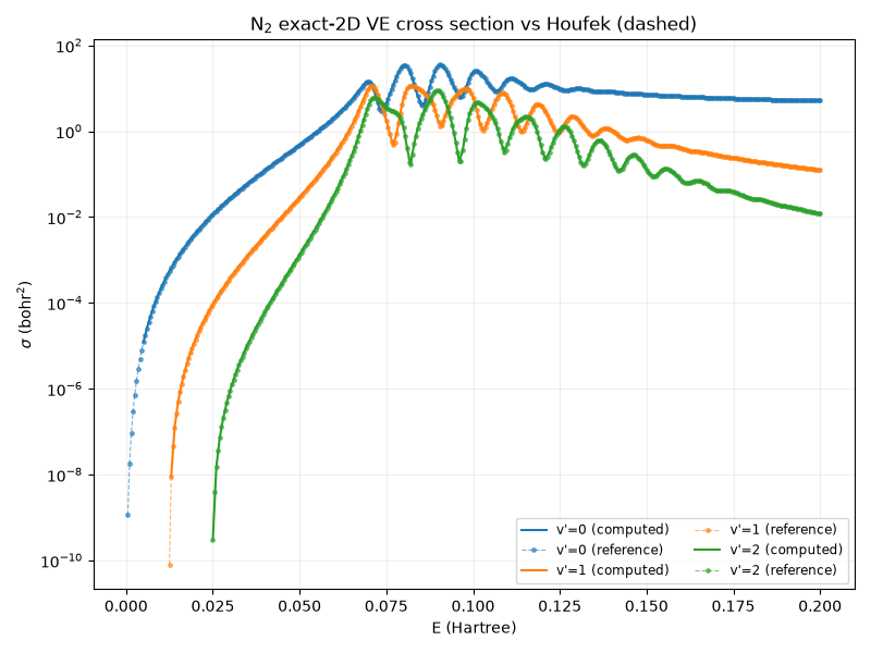
The exact-2-D curve (solid) tracks Houfek (dashed) tightly across the entire
resonance region for every plotted channel, reproducing the boomerang
oscillation structure peak-for-peak. Measured over the ~230 energies where the
two grids coincide, the median exact/Houfek ratio is 1.0000 for each of
v′ = 0, 1, 2. At the gated anchors the agreement is the same tight
differential-oracle bound the anchor sub-project established (e.g. E = 0.1 Ha,
v′ = 1: exact/Houfek = 1.000267, within GATED_RTOL = 1e-3); the two
documented-limited anchors — the elastic background (v′ = 0) at high E and the
near-threshold v′ = 1 point at E = 0.02 Ha — sit within the loose cross-model
ANCHOR_FACTOR = 3.0 band, exactly the LCP limitations #6 characterized and the
exact solver largely closes. This certifies the exact solver as a curve, not
just at isolated coordinates. plot_cross_sections is experiment-agnostic
(takes reference data as an argument, no Houfek/N₂ knowledge) so F₂/NO reuse it;
the N₂-specific, Houfek-reading driver lives on the validation/ side, keeping
projects/ free of any validation/ import.
Provenance and scope
SuperLU stays the differential oracle at every step. Core qscat remains
numpy/scipy-only; the MUMPS reuse is exercised in the Docker test image and
skips on the dev box. Deferred (each a later sub-project, unchanged from
#8’s list): complex64 + iterative refinement; MKL PARDISO as a second x86
backend; the publishing pipeline (multi-arch images, PyPI core/[mumps] extra,
wheels); a Rust non-LU kernel; interactive/HTML display; other model systems
(F₂/NO/H₂⁺) and higher-dimensional models. See
docs/physics/mumps-sparse-backend.md for the underlying backend.