Exact (non-Born-Oppenheimer) resonance states of the 2-D model

qscat.core.exact_resonance_states computes poles of the full 2-D S-matrix: eigenvalues \(E_r - i\Gamma/2\) of the complex-scaled electronic × nuclear Hamiltonian, with outgoing boundary conditions in both coordinates. No Born-Oppenheimer separation, no discrete state, no local approximation.

These are the objects qscat.core.lcp.resonance_levels approximates. Having both lets the non-adiabatic error be read directly off pole positions and widths, instead of inferred from a cross section in which many poles and a background are superposed.

Method

A resonance eigenvalue is (nearly) invariant under the ECS rotation angle while the discretized continuum rotates with it. In 2-D there are two continua — electronic (r → ∞) and nuclear (R → ∞) — each rotating with its own angle, so a state must be stable against both.

Three spectra are computed on the same model:

grid	θ_r	θ_R	what its comparison with the base tests
base	35°	35°	— (energies and states are reported on this one)
electronic-moved	44°	35°	is the state in the electronic continuum?
nuclear-moved	35°	30°	is it in the nuclear continuum?

Each spectrum comes from qscat.linalg.ShiftInvertEigs — resonances are interior eigenvalues, unreachable by a plain Krylov iteration (docs/physics/shift-invert-eigensolver.md). A state is accepted only if \(\lvert E_\mathrm{base} - E_\mathrm{partner}\rvert < \max(\mathrm{rel\_tol}\,\lvert E\rvert,\ \mathrm{atol})\) holds for both partners, and the two residuals are reported separately rather than combined into one midpoint: with two independent partners there is no single midpoint, and a state can be solid in one coordinate while marginal in the other.

Moving both angles at once would save one spectrum. It is not done, because the per-channel diagnosis is what distinguishes “no resonance here” from “the search is misconfigured” — and on N₂ that is not academic. At the resonance energy the raw spectrum is dominated by electronic-continuum × vibrational states, which the nuclear test alone accepts without complaint; only the electronic partner rejects them (they move by 2.5e-3 and 6.2e-3 Ha when θ_r changes, against ~1e-6 for a genuine pole).

Seeds are supplied by the caller. The natural source is the BO/LCP levels, but the exact solver never calls the approximation it exists to measure.

Validation: the separable limit

Switch the electronic-nuclear coupling off and the tensor Hamiltonian becomes an exact Kronecker sum,

\[H = (T_r + \mathrm{diag}\,v_\mathrm{el}) \oplus (T_R + \mathrm{diag}\,v_\mathrm{nuc}),\]

whose eigenvalues are exactly the pairwise sums \(\varepsilon_\mathrm{el} + \varepsilon_\mathrm{vib}\) of the 1-D eigenvalues on the same grids, and whose eigenvectors are exactly the products \(\phi(r)\,\chi(R)\). That is a 2-D resonance with a known position, a known width, and a known wavefunction — an oracle that a coarse grid does not weaken, because the oracle is evaluated on the identical discretization.

Measured on such a model (electronic potential frozen at R = 2.02, a Morse nuclear well):

quantity	result
pole vs \(\varepsilon_\mathrm{el} + \varepsilon_\mathrm{vib}\)	agrees to 8.6e-15
width vs the electronic width alone	agrees to rel = 1e-6
eigenvector vs \(\phi \otimes \chi\) (c-product overlap)	1 to within 1e-6
electronic residual vs the 1-D pole’s own	2.31e-07, identical
nuclear residual	~1e-17 (a bound factor cannot move)

The last two rows are the sharpest test of the two-angle bookkeeping: in the separable limit the nuclear factor is common to both electronic grids and cancels, so the 2-D electronic residual must reduce to the 1-D one, and the nuclear residual must vanish.

Result: N₂

Production deck (n_r = 107, n_R = 251, 26 857 unknowns), seeded from the first five BO/LCP levels, 118 s for the whole search on the SuperLU backend. Seven angle-stable states were found — a vibrational ladder of N₂⁻ with widths growing as it climbs, which is the boomerang picture recovered with no approximation at all.

exact \(E_r\) (Ha)	exact \(\Gamma\) (Ha)	BO/LCP \(E_r\)	BO/LCP \(\Gamma\)	\(\Delta E_r\) (meV)	\(\Delta\Gamma\) (meV)
−0.673968	0.004902	−0.673960	0.004914	−0.22	−0.33
−0.664238	0.005425	−0.664231	0.005439	−0.19	−0.38
−0.654646	0.005929	−0.654640	0.005949	−0.16	−0.54
−0.645190	0.006404	−0.645187	0.006422	−0.08	−0.49
−0.635864	0.006833	−0.635863	0.006847	−0.03	−0.38
−0.626658	0.007212	−0.626658	0.007221	−0.00	−0.24
−0.617566	0.007550	−0.617566	0.007555	−0.00	−0.14

Angle residuals across the set: electronic 1e-7–3e-6, nuclear 1e-19–5e-14.

On N₂, the Born-Oppenheimer + local approximation is excellent for the resonance levels — the differences are sub-meV throughout. Their precise size is a convergence question, answered next; the numbers in the table above are the production deck’s, and for v >= 3 they are not converged.

That verdict is specific to this observable on this molecule, and does not carry over. On σ_DA cross sections the same local approximation does poorly and in an energy-dependent way — on F₂ the LCP/exact ratio sweeps 0.263 → 1.736 across 0.010–0.050 Ha, and on NO it misses the exponential decay away from threshold entirely (see docs/physics/diatomic-ve-cross-sections.md). Reproducing where a resonance sits is a weaker demand than reproducing how much flux leaves through a given exit channel.

Converging the difference

Both sides depend on the electronic discretization — the BO levels come from an electronic pole walk — so both were recomputed at every refinement level, and it is their difference that has to settle.

Polynomial order converges at 8. Orders 8, 9 and 10 (n_complex = 6, r_max = 16) give bit-identical energies and widths to nine decimals. Order is not the limiting knob.

The real-region extent is. Holding order at 8 and growing r_max from 24 to 72 bohr (ΔE / ΔΓ in meV, exact − BO; the nuclear grid held at its converged setting throughout):

r_max	n_r	v = 0	v = 1	v = 2	v = 3
24	146	−0.217 / −0.296	−0.212 / −0.423	−0.210 / −0.610	+0.017 / −0.691
32	160	−0.226 / −0.300	−0.221 / −0.480	−0.141 / −0.626	+0.076 / −0.625
40	174	−0.221 / −0.304	−0.224 / −0.489	−0.108 / −0.642	−0.000 / −0.605
56	202	−0.225 / −0.301	−0.194 / −0.485	−0.070 / −0.439	−0.006 / −0.676
72	230	−0.220 / −0.315	−0.185 / −0.370	−0.082 / −0.602	−0.016 / −0.745

Only v = 0 is converged. It holds at ΔE = −0.22 meV (spread ±0.005) and ΔΓ = −0.30 meV (spread ±0.015) across a box grown by a factor of three.

Everything above it still moves. v = 1 looked settled at −0.22 meV on boxes up to 40 bohr and then drifted to −0.185 by 72; its width difference swings by 0.12 meV. v = 2 and v = 3 scatter more still, and their width differences wander by up to 0.2 meV with no clear limit.

Two things are worth reading off that.

The widths converge more slowly than the positions, systematically. That is expected rather than anomalous: a width measures coupling to the continuum, and growing the box changes the density of discretized continuum states the resonance is embedded in, so \(\Gamma\) keeps feeling the discretization after E_r has stopped.

And higher levels converge later, which is also the expected ordering: a higher vibrational level has a more extended nuclear wavefunction, samples the electronic potential further out, and therefore feels a truncated electronic box first.

What is established

claim	status
v = 0: ΔE_r = −0.22 meV, ΔΓ = −0.30 meV	converged over r_max 24→72
the exact pole lies below BO/LCP in both position and width	width: yes, every level, every box. Position: NOT general — on the finer 46 428-unknown deck ΔE_r turns positive at v >= 3 (see the overlap-check section)
the poles are genuine resonances, and the index pairing is correct	verified by overlap on the 46 428-unknown deck: 6/6 clean, 0/6 pairing disagreements
|ΔE_r| ≲ 0.25 meV and |ΔΓ| ≈ 0.3–0.75 meV throughout	robust in magnitude
per-level values for v >= 1	not converged — do not cite
any trend of the difference with v	not established

So the approximation puts the v = 0 state 0.22 meV too high and makes it 0.30 meV too broad, and for the higher levels all that can be said is that the sign is the same and the size is of the same order.

Two earlier readings are withdrawn. The first: on the small production deck the position difference appeared to shrink steadily with v (−0.22, −0.19, −0.16, −0.07, −0.03, …), which looked like a physical trend and was written down as one; it is largely the electronic box. The second: on boxes up to 40 bohr v = 1 appeared converged to ≲0.01 meV, and it is not — extending the box to 72 moved it by 0.04 meV in position and 0.12 meV in width. Only v = 0 survives the full sweep.

Are these poles resonances? The overlap check

Everything above rests on the poles being resonances and on the exact/BO pairing being right — and until the H₂⁺ campaign, neither was tested. Angle stability found them; angle stability is necessary and not sufficient. On H₂⁺ the same procedure produced four non-resonances out of 57 (h2plus-resonance-states.md), so this is not a hypothetical.

validation/n2/pole_verification.py runs the check with the machinery promoted out of that campaign. The result is clean:

question	answer
are the poles resonances?	yes — all 6 pair cleanly, no spurious, no weak, no box-limited
does the sorted-index pairing hold?	yes — overlap agrees at every level, 0/6 disagreements
does a bijection by energy agree?	yes — Hungarian assignment gives the same map

The reference basis is not a Rydberg series here. N₂’s anion state is a resonance, so the electronic factor comes from qscat.core.bo.resonance_curve (the two-angle pole walk, keeping the eigenvector local_complex_potential discards) and the nuclear factor from resonance_levels, combined by bo_basis_from_levels. Same comparator, different builder.

Two things the check turned up that the pole table does not show.

The overlap exceeds 1, legitimately. The c-product is a bilinear form, so Cauchy–Schwarz does not bound it. With both states c-normalized the value is just \(\lvert c(a,b)\rvert\), inflated by \(1/\sqrt{\rho_a \rho_b}\) where \(\rho = \lvert c(\psi,\psi)\rvert / \lVert\psi\rVert^2\) measures how close to real-valued a state is. The six identifications score 1.02, 1.05, 1.08, 1.11, 1.15, 1.19 — rising monotonically with Γ as ρ falls 0.66 → 0.42. H₂⁺’s narrow Rydberg resonances stay at 0.87–0.99 because they are nearly real.

Dividing by the Euclidean norms to bound it at 1 is wrong, which was measured rather than argued. That denominator weights the exponentially growing ECS tail — reintroducing exactly what the c-product’s numerator cancels, the same error as using vdot. On H₂⁺ it collapses to 0.03, 0.008 and 0.006 for three states whose node counts identify them unambiguously, and re-ranks all three onto the wrong partner. It penalizes diffuse states for being diffuse.

These poles are well localized, which is the separate question. real_weight — the fraction of |Ψ|² inside the unscaled region — is 0.96 for all six, so ρ’s fall is about the states being genuinely complex where they live, not about them leaking out of the box. On H₂⁺ the two quantities collapse together for a different reason and 18 of 57 poles come back box-limited; N₂’s do not.

The sign claim below needs narrowing. This run uses the exact_resonance_figures.py deck (46 428 unknowns), which is finer than the 26 857-unknown deck the table above was computed on. On it, ΔE_r reads −0.217, −0.212, −0.210, +0.017, +0.081, +0.081 meV — the sign flips at v = 3. ΔΓ stays negative throughout. This is consistent with the existing warning that per-level values for v >= 1 are not converged, but it is a direct counterexample to “negative at every level, on every box” as stated, and that row is qualified accordingly.

Figures

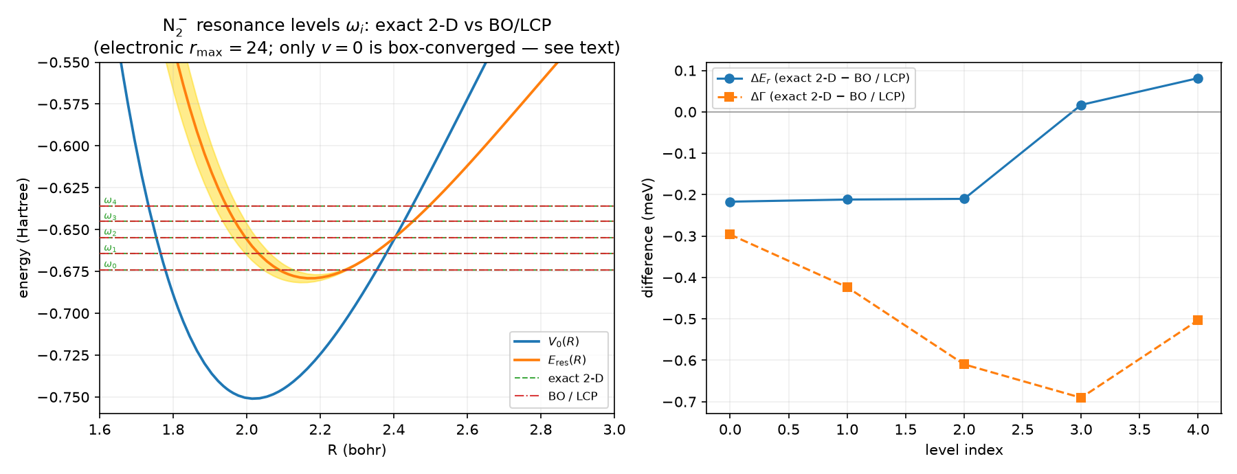
The level diagram, in the form the published version of this model uses (M. Váňa, doctoral thesis, Charles University 2017, Fig. 3.2): the neutral V0(R), the resonance curve E_res(R) with its \(\Gamma(R)/2\) envelope shaded, and the levels \(\omega_i\) drawn in that well. The published figure shows the LCP levels alone; here the exact 2-D levels are overlaid, and they are indistinguishable from the LCP ones at this scale — a fifth of a meV against a 0.2 Ha axis. That is the finding, not a defect of the plot; the right panel is where the difference lives. Both level sets come from the r_max = 24 grid, so only v = 0 is box-converged.

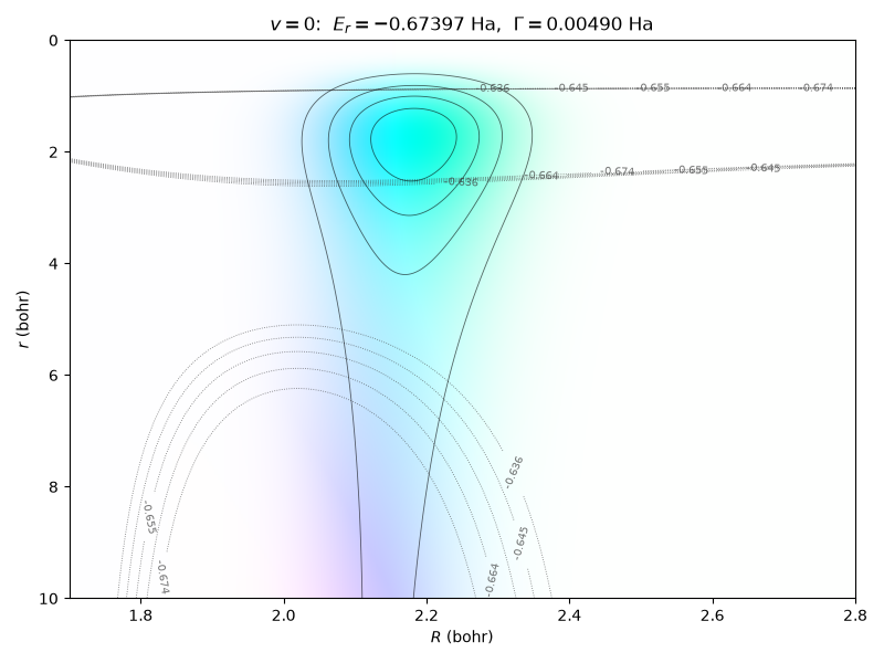
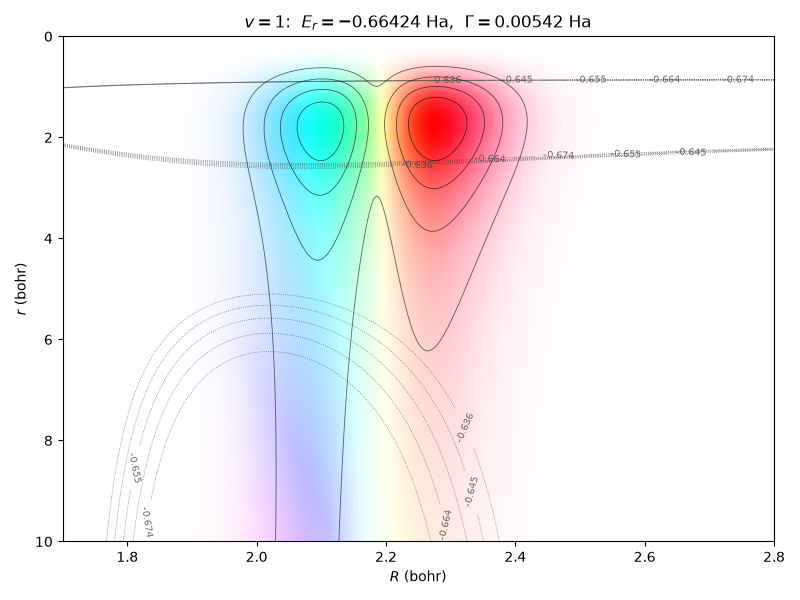
The exact resonance states \(\Psi(r, R)\) in the interaction zone, framed as the thesis’s Fig. 3.3 frames its wave-function panels (R horizontal, r vertical increasing downward, complex phase as hue, magnitude as brightness, potential contours in grey). v = 0 is a single lobe of the trapped electron at r ≈ 1–3, R ≈ 2.2; v = 1 has the expected nuclear node, visible both as two lobes in R and as the phase flip across them. v = 2 (not shown inline) carries two nodes. These are the states the BO picture approximates as products \(\phi_\mathrm{res}(r; R)\cdot\chi_v(R)\), and they are visibly close to that form here — which is the same story the 0.22 meV difference tells, in a different currency.

Brightness is one global scale across each panel, so it means the same thing everywhere in the frame. That leaves the outgoing tail faint — it is orders of magnitude below the trapped core — and the tail’s behaviour is reported numerically in the next section rather than shown. (qscat.viz.region_magnitudes can scale each region separately and does make the tail visible, but at the cost of seams at the region boundaries and a brightness that no longer means one thing across the panel; for a static figure of a trapped state that trade is not worth it.)

Regenerate with uv run python -m validation.n2.exact_resonance_figures.

Reading the phase in those panels

The obvious question on first sight of the state panels is why the phase varies at all — an eigenstate is usually pictured as real up to one global phase. Three different things are in the picture, and only one of them is phase variation.

The lobe-to-lobe colour flips are a sign, not a winding. Cyan and red sit 180° apart in hue, i.e. a factor of −1: that is a real function changing sign across a node, which is exactly what the v = 1 and v = 2 nuclear factors do.

Where the phase does wind, it must. A constant-phase wavefunction carries no probability current (\(j \propto \operatorname{Im}(\psi^*\nabla\psi)\)), and a resonance decays — \(\Gamma = 0.0049\) Ha here, a lifetime of ~200 a.u. — so it has to carry outgoing electronic flux, and flux requires a phase gradient. A resonance eigenstate of constant phase would be a bound state.

Both statements are measurable. Rotating each state by the single global phase that makes it maximally real and then measuring the residual imaginary weight \(\|\mathrm{Im}\,\psi\| / \|\psi\|\) in shells of r (0 means real up to a constant phase, 1/√2 means a pure traveling wave):

state	\(\Gamma\) (Ha)	r ∈ [0,4)	[4,10)	[10,16)	[16,24)
v = 0	0.00490	0.146	0.434	0.799	0.702
v = 1	0.00542	0.249	0.502	0.718	0.707
v = 2	0.00593	0.309	0.545	0.686	0.713

The core is nearly real — 85% for v = 0 — and the tail saturates at 0.707, the traveling-wave value. So the state is quasi-bound where it is bright and purely outgoing where it is faint, which is what a resonance is. The winding rate measured along r (0.21–0.33 rad/bohr) sits just below the single-channel estimate Re k = √(2E) (0.39–0.44), as it must: the state decays into several open vibrational channels at once, each with its own momentum, so a single cut shows their mixture.

None of this is an ECS artefact. Inside the real region the ECS map is the identity, and R0 = 24 bohr while the panels show r <= 10, so what is plotted is the physical Siegert wavefunction. ECS’s contribution is to make the state findable at all: Im k ≈ −0.006 means that outgoing tail grows as e^{+0.006 r} — the Siegert divergence — and rotating the contour past R0 turns that growth into decay, so the state becomes a square-integrable eigenvector.

One convention note: after c-product normalization (\(\psi^T\psi = 1\), not \(\psi^\dagger\psi = 1\)) the residual freedom is only ±1, so relative phase across the panel is meaningful but the absolute hue is not.

The reality defect also tracks the widths — 14.6%, 24.9%, 30.9% against \(\Gamma\) = 0.00490, 0.00542, 0.00593. Higher levels are more strongly coupled to the continuum, so they are less quasi-bound and less real, which is the same physics that makes their BO/exact differences converge more slowly than v = 0’s.

A caveat on the BO side: resonance_levels emits a warning for this model that \(\Gamma(R)\) is nonzero where the anion curve lies below the neutral, i.e. where autodetachment is closed, so the BO widths carry their own documented qualification (see docs/physics/lcp-resonance-levels.md).

Limits

• Validated on N₂ and H₂⁺. H₂⁺ (Coulomb, with a Rydberg series accumulating at each threshold) is covered in h2plus-resonance-states.md. F₂/NO — where the dissociative channel is open, so the nuclear residual becomes the informative one — have not been run.

• The two-angle test is necessary, not sufficient. A small residual says the eigenvalue did not move when the contour did — and a rotated-continuum state sitting in a stable corner produces that too, as four of H₂⁺’s 57 poles did. A grid too coarse to resolve a state can produce it for a third reason. Four separate checks answer four separate questions: overlap against a BO basis (qscat.core.assignment.pair_by_overlap) for “is this a resonance”, real_weight for “does the box still hold it”, grid refinement for “is the discretization adequate”, and the residuals here for “did the contour move it”. The overlap is blind to the second by construction — the c-product cancels the rotated tail — so a state 97 % outside the box still pairs at 0.99. On H₂⁺ that blindness hid 18 poles.

• Seed placement matters more than it looks. k eigenpairs nearest a shift is a local window: with a vibrational spacing of ~0.0096 Ha, a seed one quantum away returns v = 1 and v = 2 while v = 0 falls off the end of the list. The search then reports real states that are not the ones asked for.

• The acceptance tolerance is a statement about the grid. The default rel_tol = 1e-4 can only be met if the electronic grid resolves the pole to better than that between angles. On a grid with order = 5, r_max = 12 the 1-D pole is angle-stable only to 7e-4, and every resonance is rejected — correctly, in the sense that the grid cannot support the claim.

• Cost is one sparse factorization per (grid, shift): three grids × the seed count. At 26 857 unknowns that is ~8 s each on SuperLU, and ~26 s at the 55 332 unknowns of the r_max = 40 convergence deck; the MUMPS backend is the route to larger decks.

• Only v = 0’s difference is converged. v >= 1 still moves at r_max = 72 bohr — in width especially — so those per-level numbers are indicative of sign and order of magnitude only.