H₂⁺ dissociative recombination (the first ionic model)¶
Location: the ionic pieces live in qscat (qscat.special.coulomb, qscat.model.H2P /
IonicResonanceModel, qscat.core.dr_cross_section); the deck + validation in
validation/h2plus/ (config.py — the eMoScat deck definitions, kept as the tuner’s reference +
the qscat-run deck-parity guard test_config.py; the exact σ_DR curves now run through
apps/qscat-run). The DR convention gate (c-product vs eMoScat’s conjugated dot) lives in
libs/qscat/tests/test_dissociation.py.
Origin: sub-project D of the DA/DR design spec
(docs/superpowers/specs/2026-07-27-da-cross-sections-design.md), designed in
docs/superpowers/specs/2026-07-28-h2plus-dr-design.md and ported from eMoScat via port-scout.
Units: atomic units.
Key result¶
The exact-2D TI \(\sigma_\mathrm{DR}(E)\) for e⁻ + H₂⁺ is delivered at full
deck size — ~1.15 M unknowns on the 1300-bohr Coulomb electronic grid —
through apps/qscat-run under Docker/MUMPS at ~8 s/energy: the DR1 (n=0)
channel peaks at E ≈ 6.31×10⁻³ Ha, σ ≈ 1.54×10⁻³ bohr² above a ~10⁻¹⁰
background; DR2 (n=1) is ~10⁻⁶; DR3 (n=2) is closed in the window
(threshold ≈ 0.0426 Ha). Against a previously obtained reference sweep,
DR₀ agrees once a measured 2π normalization convention is accounted for
(geometric mean 1.001), while DR₁ carries a systematic ~1.3× deficit that
remains an OPEN, documented discrepancy — the narrative below records what
was ruled out, and why the Born-Oppenheimer levels are where the agreement
is genuinely readable.
What this is — and why it is different¶
Everything before H₂⁺ was neutral electron–diatomic scattering. H₂⁺ is an ion: the scattering electron sees the +1 core charge, i.e. a long-range −1/r Coulomb tail. That one fact changes three things:
The channel functions become Coulomb, not free Riccati-Bessel. The incident wave is a long-range Coulomb wave — so the electronic grid must reach ~1300 bohr.
The process is dissociative recombination (DR):
e⁻ + H₂⁺(v) → H + H. The electron is captured into a Rydberg resonance of the neutral H₂, which dissociates on the neutral curve.There is a Rydberg series of exit channels (the neutral’s bound electronic states, accumulating at the −1/r continuum edge), cut off at a measurable number (
N_CHANNELS = 3).
This is deliberately the first non-laptop-scale model — the full 2-D deck is ~1.15 million unknowns (see Discretization). It targets the Docker/MUMPS path; the test suite validates it analytically and on a reduced proxy.
Coulomb special functions (qscat.special.coulomb)¶
The charge-z generalization of riccati_bessel_en/riccati_hankel_en. Energy-normalized regular /
irregular / outgoing Coulomb functions, Sommerfeld parameter \(\eta = m z / k\), argument \(\rho = k x\):
with \(G^\mathrm{en}\) defined likewise.
Backed by mpmath (coulombf/coulombg), which accepts complex ρ — required for
ECS-rotated arguments. At \(z=0\), \(F_l(0,\rho) = \rho\,j_l(\rho)\), so coulomb_f_en(·,·,0,m,l) reduces
EXACTLY to riccati_bessel_en (mass m) — the direct differential-test hook, verified to ~1e-16.
(Note: coulomb_h1_en(z=0) = i·riccati_hankel_en, since \(G_l(0,\rho) = -\rho\, y_l(\rho)\) while \(F_l = +\rho\, j_l(\rho)\)
give \(G + iF = i(j_l + i y_l)\rho\) — the code keeps the physical H⁺=G+iF; only the test carries the
i.) Two eMoScat gotchas were NOT replicated: its sH1 wrapper had a copy-paste bug (returned F,
not G+iF), and its wrappers ignored coulcc’s ifail.
The ionic model (qscat.model.H2P)¶
The model layer was generalized for ions: the ResonanceModel protocol gained a charge
attribute (0 for the neutral diatomics — unchanged — and −1 for H₂⁺) and shed the engine-unused
lam. H2P is an IonicResonanceModel with the extracted eMoScat form (μ=918.076, ℓ=1,
charge=−1):
Reduced mass. μ=918.076 is mₚ/2 for the modern proton mass (1836.15267/2), as given by three independent published sources: D. Hvizdoš, Two-dimensional model of dissociative recombination, master’s thesis, Charles University 2016, Table 1.1 (the first time-independent solution of this model, which the present
dr_cross_sectiondescends from); Váňa 2017 Table 1.2; and Hvizdoš et al., Phys. Rev. A 97, 022704 (2018) §II A. eMoScat’s JSON deck carries 918.25, which both publications contradict; the port originally inherited that value and it was corrected on 2026-08-15. The 0.019% shift moves H₂⁺ vibrational spacings by ~1e-4 relative — immaterial qualitatively, but wrong for reproducing published numbers.
ion Morse \(v_0(R) = V_0\left(e^{-2\alpha(R-R_0)} - 2e^{-\alpha(R-R_0)}\right)\), with
V0=0.1027, R0=2.0, alpha=0.69(the initial vibrational state lives here; the1/Rproton repulsion is folded into this single Morse, not explicit);σ-capture
v_int(r,R) = −a₁(1−tanh Q(R))·S(R)·(e^{−r²/3}/r),Q=(a₂−R−a₃R⁴)/7,S=tanh(R/a₄)⁴,a₁=1.6435, a₂=6.2, a₃=0.0125, a₄=1.15;surface \(= v_0(R) + v_\mathrm{int}(r,R) + \ell(\ell+1)/2r^2 + \mathrm{charge}/r\) — the
charge/r = −1/ris the ionic electron–core Coulomb attraction.
Adding an ion is data + validation, no engine changes (the same lesson as the neutral molecules).
The DR cross section (qscat.core.dr_cross_section)¶
dr_cross_section is da_cross_section generalized, reusing v_dr_diag,
anion_electronic_states, riccati_bessel_en_mass, and the driven Lippmann-Schwinger sweep. The
only new physics is (a) a Coulomb incident (channel_vector(..., charge=−1)) and (b) a loop
over the Rydberg exit channels instead of one anion state:
\(\Psi_+ = \Psi_i - (E_\mathrm{tot}\mathbb{1} - H_\mathrm{2D})^{-1} V_\mathrm{int} \Psi_i\), \(E_\mathrm{tot} = E + \varepsilon_{v_\mathrm{init}}\), Coulomb \(\Psi_i\) (potentials on the complex ECS coordinate — eMoScat’s real-part
// FIXMEis fixed);Rydberg states \(\phi_e^{(n)}\),
E_ryd(n) = eps_e^(n)fromanion_electronic_states(…, n_states=N)(they are bound below the −1/r continuum — the same bound-state solver);\(V_\mathrm{DR} = V_\mathrm{int} + v_0(R) - V_\mathrm{int}(r,R_\infty)\) (the rearrangement interaction);
per open channel \(n\) (\(E_\mathrm{tot} > E_\mathrm{ryd}(n)\)): \(T_n = \langle \phi_e^{(n)} F^\mathrm{nuc}_{K_n,0} \,\vert\, V_\mathrm{DR} \,\vert\, \Psi_+ \rangle\) (c-product), \(\sigma_n = 4\pi^3|T_n|^2/2E\).
The c-product is the ECS-correct choice where eMoScat used a conjugated dot (zdotc); the
port validates they agree — the relative difference is ≈3.4×10⁻¹² on the proxy (the
rotated-nuclear-tail contribution is negligible there), so the convention question is settled.
Discretization (fem_grid_exp_tail, validation/h2plus/config.py)¶
The Coulomb tail forces a huge electronic grid. A new builder fem_grid_exp_tail (like
segmented_grid but with an exponential-growth ECS tail — reusing the _ecs_tail helper) builds
the eMoScat deck:
real region |
ECS tail |
2-D size |
|
|---|---|---|---|
electronic |
→ 1300 bohr (n=1406) |
5°, exp-growth ×25 |
|
nuclear |
→ 14 bohr (n=818) |
22°, exp-growth ×25 |
~1.15 M unknowns |
That is firmly Docker/MUMPS territory — not laptop-runnable. config.proxy_grid() (electronic
→60 bohr) and an even smaller test grid give a laptop-feasible well-posedness/threshold gate,
not a converged cross section.
What a full-deck energy point costs (measured)¶
Measured 2026-08-17 on an x86-64 host (32 cores, 123 GB) under MUMPS, via
apps/qscat-run/examples/h2p-dr-probe.yaml:
quantity |
value |
|---|---|
unknowns / nonzeros |
1 150 108 / 19 507 356 |
|
34.80 s → 17.4 s/energy |
grid build + vibrational states |
0.42 s |
peak RSS (from an earlier 50-energy sweep) |
4.34 GB |
So a σ(E) sweep costs roughly 1 hour per 200 energies. Over 0.023 Ha of energy windows that is ~2.2 h at 5e-5 Ha spacing, ~5.6 h at 2e-5, ~11 h at 1e-5 — an overnight job rather than the multi-day one the size suggests.
Two caveats worth carrying. Earlier ad-hoc sweeps on the same host recorded
12.4–14.1 s/energy, so treat those as a lower bound and budget on 17.4. And
the memory figure is comfortable only because MUMPS is used: the SuperLU path on
a deck an order of magnitude smaller already needed 7.4 GB
(docs/physics/mumps-sparse-backend.md).
The converged full-size σ_DR(E) curve (delivered)¶
The exact-2D TI σ_DR(E) now runs through apps/qscat-run (config-driven — the per-molecule DR
driver was retired in the qscat-run consolidation). The H2P emoscat preset grid is byte-identical
to the retired driver’s full_grid (locked by
validation/h2plus/test_config.py::test_h2p_decks_match_presets), so qscat-run reproduces its data
exactly. Run the full 1300-bohr deck under MUMPS via
apps/qscat-run/examples/h2p-dr-ti.yaml (methods: [ti], observables: [{kind: dr, channels: 3}],
grid: {preset: emoscat}):
docker/run.sh apps/qscat-run/examples/h2p-dr-ti.yaml runs/h2p-dr-ti
The committed figure docs/physics/figures/h2plus-dr-cross-section-shortrange.png is the log–log
short-range accuracy view (narrow the config’s energies to a fine sweep across the DR1 resonance
in [0.005, 0.007] Ha to reproduce it):
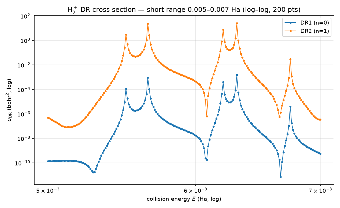
The DR1 (n=0) channel peaks at E ≈ 6.31×10⁻³ Ha, σ ≈ 1.54×10⁻³ bohr² above a ~10⁻¹⁰
background; DR2 (n=1) is ~10⁻⁶; DR3 (n=2) is closed in this window (threshold ≈ 0.0426 Ha). The
solve runs in ~8 s/energy on the sadaharu host with the OpenMP MUMPS backend.
Against a previously obtained reference sweep¶
A prior 5001-point σ_DR(E) sweep of this model, together with the author’s own Born-Oppenheimer level table, exists outside the repository. Both were used to check this implementation, and they gave very different quality of answer — for a reason worth recording, because it decides how this observable can be validated at all.
The normalization¶
The reference σ values carry a \(2\pi\) this repository does not. That was measured, not assumed: the ratio reference/computed is 5.3–7.2 on DR₀, clustering on \(2\pi = 6.283\) — not on 1, and not on \((2\pi)^2 = 39.5\). Across the sampled points its geometric mean on DR₀ is 1.001, so the constant is confirmed to ~0.1%. (The corresponding VE convention differs by \((2\pi)^2\).)
DR₁ carries a systematic deficit — an open discrepancy¶
Twelve energies have been compared, in two batches: six chosen on resonance structure and six chosen for flatness (below). Splitting the residual by channel separates two different effects, and only one of them is benign.
channel |
geometric mean |
spread |
points below 1 |
|---|---|---|---|
DR₀ |
0.980 |
0.847–1.152 |
4 / 9 |
DR₁ |
1.295 |
0.983–1.804 |
1 / 9 |
(excluding three points within 1e-3 Ha of a vibrational threshold, treated below)
DR₀ scatters symmetrically about 1 — that is the position sensitivity described in the next section, and it is not a defect.
DR₁ does not. Eleven of twelve points lie above 1 and the twelfth is 0.983. A resonance-position difference moves a ratio in both directions, since our resonance can fall on either side of the reference’s; it cannot produce a one-sided residual. So σ_DR₁ computed here is systematically ~30% below the reference, and that is unexplained — it should be treated as an open discrepancy in this channel, not as agreement.
What is ruled out:
A global constant — DR₀ would be shifted with it, and it is not.
The level positions and thresholds — ≤4e-6 Ha and µHa respectively (below).
A channel-indexing mismatch. The published
DR_1really is this implementation’seps_ryd[1], pinned by the third channel:ch2opens here at 0.042742 Ha and the reference’sDR_2column turns on at 0.042803, so the columns line up one-for-one.Degenerate states being grouped into one published column. The exit series is measured clean —
n_eff= 0.60, 2.00, 3.02, 4.02, 5.02, 6.02 with a smallest gap of 6e-3 Ha — so there is no near-degenerate pair for the reference to be summing where this implementation takes one state.
The offset is flat in energy, which narrows what it can be. An error in the
exit-channel normalization would most naturally enter through
k_r = sqrt(2 mu e_dr), and e_dr for this channel varies by 80% across the
compared range (0.028→0.064 Ha) — so a k_r-dependent mistake would show up as
a trend. It does not: regressing log(ratio) on log(k_r) gives correlation
+0.11 and an implied power of +0.18, i.e. no dependence, and on
log(E) correlation −0.01. The residual behaves as a constant factor of
~1.3 applied to channel 1 alone, with the symmetric position scatter
superposed on top of it (4 of 11 points fall below 1.295, 7 above).
So the thing to look for is a channel-specific constant — a normalization or
weight attached to the exit state — rather than an energy-dependent
normalization error. eMoScat’s per-Rydberg-state deck rydbergs.txt is not in
this repository’s reference snapshot, so the published per-channel convention
cannot be read off directly and this has to be settled against the source.
Near a threshold σ_DR runs high, and badly so. This is the larger of the two problems and probably the more urgent.
At E=0.009543, 2.6e-4 Ha below the v=1 vibrational threshold, this
implementation gives 7.6× (DR₀) and 3.7× (DR₁) MORE than the reference. All
three of the twelve compared points that lie within 1e-3 Ha of a vibrational
threshold are outliers, all in that direction.
The same failure appears far more starkly in the third Rydberg channel, which
is barely open over the whole range where it can be compared at all
(apps/qscat-run/examples/h2p-dr-channel-probe.yaml, three energies just above
its 0.0427 Ha opening):
E (Ha) |
ours |
reference / 2π |
ratio |
|---|---|---|---|
0.045259 |
1.35e-4 |
1.95e-7 |
0.0014 |
0.047465 |
3.24e-6 |
2.93e-7 |
0.090 |
0.049122 |
2.14e-5 |
6.81e-7 |
0.032 |
So σ_DR₂ here is 100–700× too large and non-monotonic where the reference rises smoothly. That is a qualitative failure, not a normalization offset, and it cannot be position sensitivity at that magnitude.
The variable is exit momentum, not diffuseness. That probe was designed to
test whether the DR₁ offset scales with how diffuse the exit state is (ch2 has
n_eff 3.02 against ch1’s 2.00), and it does not — the ratios do not order by
n_eff at all. What does order is k_r = sqrt(2 mu e_dr): ≈49 for ch0
(ratio 1.08), ≈10 for ch1 (1.26), and ≈2–3 for ch2 (0.016). A channel
evaluated close to its own threshold, where k_r is small, is where this
implementation departs — consistent with the vibrational-threshold outliers
above, which are the same condition reached a different way.
That makes the near-threshold exit-channel treatment — riccati_bessel_en_mass
and its energy normalization at small k_r — the concrete thing to examine,
and it is a different defect from the flat DR₁ factor below.
Why pointwise σ(E) is also position-limited¶
Beyond the DR₁ offset, the residual has a second component that IS benign and that bounds how well any pointwise comparison can do:
The DR resonances are narrow. Across the reference sweep there are 80 prominent DR₁ peaks with a median FWHM of 2.0e-5 Ha, and 54 of them are narrower than two of the sweep’s own 1e-5 Ha samples. The reference curve does not fully resolve its own structure, and neither would any sampling at that spacing.
This repository’s level positions agree with the reference’s to a few µHa (below). On a 2e-5 Ha Lorentzian evaluated on its flank, a 3e-6 Ha position difference changes σ by ~26% — the observed scatter, from agreement that is otherwise excellent.
So sampling σ at a structured energy measures position agreement, amplified,
and reports it as a cross-section disagreement. Independent corroboration of
the width scale: the exact 2-D poles computed here (validation/h2plus/exact_poles.py)
come out at Γ ≈ 1e-7–2e-5 Ha, the same scale as those measured peak widths.
A comparison energy therefore has to be chosen for conditioning, and “smooth”
judged by a finite difference at the reference’s own 1e-5 spacing does not
qualify, since most peaks are unresolved there.
apps/qscat-run/examples/h2p-dr-validation.yaml selects the flattest energies in
the sweep instead: each varies by under 15% (the best under 2%) across ±6e-5 Ha —
20× the position agreement — in both open channels at once.
That selection is necessary but demonstrably not sufficient, and the honest record of this is that choosing flat energies did not tighten the residual: the flat batch spread 0.13–1.80 against the structured batch’s 0.85–1.57. Flatness alone does not screen out threshold proximity, and it does nothing at all about the DR₁ offset above, which is not a conditioning problem. The remaining conclusion is that pointwise σ_DR is a poor validation instrument for this model whatever energies are chosen — which is why the level table below, not this comparison, is what the repository gates on.
Where the agreement is readable: the levels¶
The well-conditioned check is against the published \(\omega_i^j\) level table, which is
the same physics without the amplification. All 53 published levels — 5 for
Ry_0, 12 each for Ry_1…Ry_4 — agree to ≤4e-6 Ha, gated in
validation/h2plus/test_rydberg_levels.py against
validation/h2plus/reference_levels.py.
That residual is itself accounted for, and it is not discretisation. Swapping in
eMoScat’s reduced mass 918.25 for this repository’s 918.076 drops the mean
level difference from 2.4e-6 to 1.1e-7 Ha — so the published table was
computed with 918.25, and one constant explains essentially all of it. The
918.076 here is deliberate and better sourced (Váňa 2017 Table 1.2, Hvizdoš
2016 Table 1.1, Hvizdoš et al. 2018 §II A all give m_p/2 = 918.076, which
eMoScat’s deck contradicts). At matched constants this implementation
reproduces the published levels to ~1e-7 Ha.
The electronic grid near the origin¶
Worth stating explicitly, because the potential looks alarming there. At
R = 14 bohr — the R_inf that sets the exit channels — surface(r, R) has a
deep, narrow well: −4.11 Ha at r = 0.446 bohr, with a steep l = 1
centrifugal wall inside it (V(0.01) ≈ +9.8e3 Ha ≈ 1/r², a classically
forbidden region the wavefunction is exponentially suppressed in).
That well sits inside the innermost grid segment, which this repository
transcribes from eMoScat’s H2p.json verbatim: 10 elements of 0.1 bohr over
[0, 1] at dvr_order = 8, i.e. ~0.014 bohr between DVR points. Against the
shortest de Broglie wavelength in the well (2.69 bohr for the deepest channel)
that is ~190 points per wavelength, 0.037 wavelengths per element — heavily
over-resolved rather than marginal. The empirical confirmation is the level
table above: those levels are eigenvalues of exactly this electronic
Hamiltonian on exactly this inner grid, and they reproduce the published values
to ~1e-7 Ha at matched constants. The near-origin discretisation is not a
source of error here, and in particular is not a candidate for the DR₁
deficit.
Two further position checks agree independently:
Check |
Agreement |
|---|---|
Cation vibrational thresholds |
1–4 µHa |
Third Rydberg channel opening |
ours 0.0428, reference 0.042803 Ha |
That last one also confirms the channel bookkeeping: ch2 is identically zero
below 0.0428 Ha in this repository, and the reference’s DR₂ column is likewise
zero until 0.042803.
Coulomb functions: z→0 reproduces
riccati_bessel_en/riccati_hankel_en(~1e-16); a known mpmath value; finite on complex ECS arguments.The model:
v0/v_int/surfacematch the extracted formulas;charge=−1; the neutrals keepcharge=0andchannel_vector(charge=0)is byte-identical to before.DR (small proxy,
@slow): σ_DR finite, ≥0, correctly shaped; a genuinely closed Rydberg channel returns exactly 0 (the 3rd channel, threshold ≈0.0426 Ha, above the probe energies); and the c-product vs conjugated-dot agreement (≈3.4e-12) justifies the convention. This is a well-posedness gate, NOT a converged σ_DR — the real grid is 1300 bohr.Docker/MUMPS: the exact σ_DR(E) is a full-deck (~1.15 M unknown) solve — Docker/MUMPS only. No independent golden data ships (eMoScat’s
output/H2+/sigma.txtis absent from the snapshot), so — as for the neutral DA — the exact solver is the oracle. The converged curve is delivered — see “The converged full-size σ_DR(E) curve (delivered)” above.
The resonance positions behind these peaks¶
Where the peaks in this cross section come from – the exact 2-D poles, the
Born-Oppenheimer levels they are conventionally assigned to, the wavefunctions
of both, and the four angle-stable states that turn out not to be resonances –
is h2plus-resonance-states.md. That note also uses this sweep as its
measuring instrument: the poles land on its peaks to 0.2-0.3 resonance widths.
Follow-ons¶
The π channel (p_pi_potential); optimizing the mpmath Coulomb functions (a Rust/COULCC port) if
they become the bottleneck; rotational / coupled-channel (non-adiabatic) DR.