N₂ — the benchmark target¶
N₂ is the only molecule in this repository with independent published data
to check against: Karel Houfek’s CSVE.V00.J00 vibrational-excitation cross
sections. Everything else — NO, F₂, H₂⁺ — is validated against qscat’s own
exact solver. That makes N₂ the anchor: the solver earns the right to act as
an oracle elsewhere by matching Houfek here.
The model itself is a given testbed, not a claim about the real molecule: agreement with Houfek certifies this repository’s numerics, since Houfek’s calculation is an independent implementation of the same fixed-nuclei ²Π_g shape-resonance surface and method — not the model’s physical realism. Once certified, the exact 2-D solver becomes the oracle other approximations (the 1-D local-complex-potential reduction, the nonlocal resonance model, Born–Oppenheimer resonance levels) are measured against.
Atomic units throughout (Hartree, bohr).
The model — form and parameters
qscat.model.N2 is a DiatomicResonanceModel with charge = 0: the shared
neutral-diatomic form, a Morse neutral curve plus a sigmoid-and-Gaussian
resonant interaction, fixed at partial wave ℓ = 2. Values printed directly
from the model object:
parameter |
value |
|---|---|
|
12766.36 |
|
2 |
|
0.75102 |
|
1.1535 |
|
2.01943 |
|
6.21066 |
|
1.05708 |
|
−27.9833 |
|
5.38022 |
|
2.405 |
|
0.4 |
|
0 |
Reproduce these with:
from qscat.model import N2
print({k: v for k, v in vars(N2).items() if not k.startswith("_")})
Parameters are from M. Váňa’s doctoral thesis (Charles University, 2017),
which also publishes the LCP formulation this model’s resonant term follows;
see reference/literature/vana-2017-thesis.md for the tracked reference
note. The model’s neutral vibrational spacing (eps1 - eps0 ≈ 0.0124 Ha) is
about 16% larger than real N₂’s spectroscopic value — a deliberate, accepted
property of the extracted model, not a numerics bug (carried through every
number below).
What has been computed¶
The exact 2-D driven Lippmann–Schwinger solve. 4 of 6 anchors are GATED
against Houfek at GATED_RTOL = 1e-3, which sits ~3.7× above the largest
deviation actually observed — and at every one of them the exact solver is
3–5 orders of magnitude closer to Houfek than the LCP is. The other 2 (elastic at E=0.2 Ha; near-threshold v’=1 at E=0.02
Ha) are reported as NOTE rather than gated — for continuity with the LCP’s
own anchor exclusions — but the exact solver actually matches Houfek there
too, to within 7.5e-07 and 2.3e-04 relative deviation respectively,
resolving both of the LCP’s known structural gaps.
Figure: ../physics/figures/n2-2d-ti-cross-section.png.
Wavepacket propagation reaching the same cross section by an independent
route — and why order-1 Crank–Nicolson was not good enough to get there
(~100% accumulated error) while order-3 Padé matches the TI oracle to
~1–2% median across 0.04–0.18 Ha. Needs an elastic free-reference
subtraction to avoid a ~500× spurious background in the diagonal channel.
Figure: ../physics/figures/n2-2d-td-vs-ti-vs-houfek.png.
The 1-D reduction: 4 of 6 anchors agree with Houfek within a factor-of-3 band (ratios 0.445–0.826 at E=0.2 Ha, v’=1–3; 1.010 at E=0.1 Ha, v’=1). The other 2 are documented, structural limitations — the elastic channel omits non-resonant background scattering (ratio 0.040) and the fixed local width gives the wrong near-threshold law (ratio ~8133 at E=0.02 Ha).
Poles of the full 2-D S-matrix: seven angle-stable N₂⁻ states, a
vibrational ladder with widths growing as it climbs. Only v=0 is
box-converged (ΔE_r = −0.22 meV, ΔΓ = −0.30 meV vs. the Born–Oppenheimer
levels); higher levels are not converged, and the position difference’s
sign is not general — it turns positive at v ≥ 3 on a finer grid.
Overlap-verified: 6/6 clean, 0/6 pairing disagreements.
Figure: ../physics/figures/n2-exact-2d-resonance-levels.png.
The nonlocal resonance model¶
The nonlocal resonance model (NRM) is a different approximation from the
LCP: instead of reducing the resonance to a local complex potential, it
keeps the full nonlocal coupling of PRA 77’s Feshbach formalism, expanded
in a discrete-state basis. Measured against the exact 2-D solver
(qscat.core.driven.ve_cross_section as oracle) at 11 energies over
0.06–0.16 Ha, v_init = 0:
Choice B (R-independent discrete state) with the Eq. (37) background reproduces the exact cross section to better than 0.7% in both the elastic (0→0, ratio 0.99883–1.00019) and first inelastic (0→1, ratio 0.99706–1.00065) channel.
Dropping the background term, or using choice A (the physical, R-dependent discrete state), widens the spread substantially (choice B without background: 0.517–1.338; choice A with background: 0.854–1.059 pooled across channels).
The LCP, by contrast, spans 0.106–4.568 over the same comparison — the NRM’s nonlocal treatment closes most of the gap the 1-D reduction leaves open in vibrational excitation, on this molecule.
These ranges are bands over the 11 recorded energies, not over every energy in the plotted window — the denser figure grid widens two of them further (§9 of NRM vibrational excitation quantifies it).
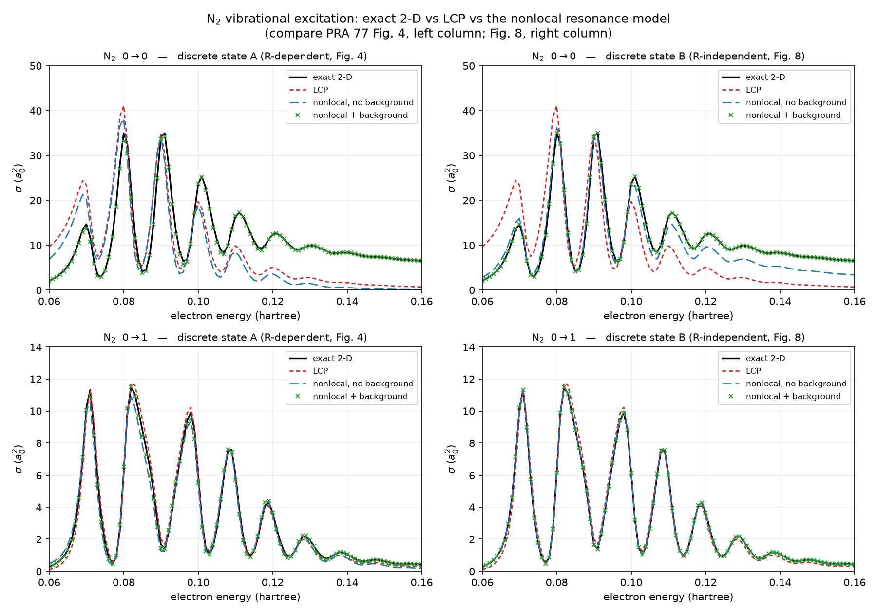
Rows are the transitions (0→0 top, 0→1 bottom); columns are the discrete-state choice (A left, B right). Full derivation and validation ladder in NRM vibrational excitation.
Where to read more¶
The exact 2-D solver and its time-dependent twin: N₂ vibrationally-elastic/inelastic cross section: exact 2-D driven-equation method, N₂ vibrationally-elastic/inelastic cross section: time-dependent (Crank-Nicolson) route to the exact 2-D solution. The 1-D LCP reduction and the electronic resonance pole it is built from: N₂ vibrationally-elastic/inelastic cross section: TI resolvent/driven-equation method, N₂ electron-impact ²Π_g shape resonance: fixed-R pole search. The earlier, dense-solver time-dependent route (a stepping stone to the 2-D TD method above): N₂ vibrationally-elastic/inelastic cross section: time-dependent (Crank-Nicolson) method. Exact, non-Born-Oppenheimer resonance states: Exact (non-Born-Oppenheimer) resonance states of the 2-D model. The nonlocal resonance model: The nonlocal resonance model (NRM), and its vibrational-excitation route: NRM vibrational excitation. The three alternative time-dependent energy-extraction routes (Tannor-Weeks, delta, flux), validated on this same model: Alternative TD energy extractors: Dirac (delta) and Flux (flow).