Coupled partial waves in the NO shape resonance: does the fixed-l reduction hold?

Location: projects/no_coupled_channels/ (anisotropy.py, model.py, blocks.py, angular.py, scattering.py) for the coupled-channel model and its cross-section solver, plus renormalised.py (the well whose lam is rescaled to preserve the anion curve); validation/coupled/ (screen.py, observable.py, energies.py, cross_section.py, figures.py, renormalise.py, per_ell_curves.py, s0_control.py, bound_count.py, renormalised_campaign.py, symmetric_run.py) for the pole campaign, the normalisation solve, the per-wave scan, the controls and the figures. Origin: a coupled-channel extension of qscat.model.NO’s local complex potential (LCP) model — the shipped model represents the anion shape resonance with a single partial wave (Lambda = 1), and this project asks whether that reduction still holds once a physically motivated, non-spherical interaction is allowed to couple it to neighbouring partial waves. Units: atomic units throughout (energy in Hartree, length in Bohr, cross section in bohr²). Every matrix here is complex symmetric (ECS), never Hermitian.

Key result

The question. The shipped NO model represents the anion shape resonance with a single partial wave. Does that reduction survive once a non-spherical interaction couples it to neighbouring waves?

The answer, for the vibrational-excitation cross section: yes, and for a reason that is not specific to this model. A low-energy electron cannot resolve the anisotropy. At the resonance energies here the wavenumber is \(k \approx 0.45\) a.u., so the electron’s wavelength is about 14 bohr against a well displacement \(d = sR/2 \approx 0.33\) bohr at equilibrium — a factor of 40. Measured, less than 0.1 % of the cross section leaves the entrance partial wave (max 0.19 %, at the top of the energy range where \(kd\) is largest). Coupling that weak cannot move an angle-integrated cross section much, and the residual effect is being measured now (see Open below).

Six things are established.

1. Only \(l = 1\) hosts a resonance. Over eight values of \(R\), three different wells, and a window reaching 3.8 Ha above the neutral with \(\Gamma\) up to 1.2 Ha, the \(l = 2, 3, 4, 5\) blocks contain no angle-stable pole at all (validation/coupled/per_ell_curves.py). This is the atomic physics showing through: O\(^-\) has exactly one bound orbital, \(2p\), and binds nothing in \(s\) (no Coulomb tail, so no Rydberg series) or in \(d\) (the centrifugal barrier against a neutral core). The higher waves are INERT — the \(l = 1\) resonance can only leak into them and back out.

2. That explains the single-pole null. No second pole ever appears in the screen because no channel is able to host one. This is a mechanism, which is a stronger statement than a search that found nothing.

3. Splitting the well destroys the dissociation limit. The two centres share lam as \((1\pm\kappa)/2\), so the deeper well keeps only part of it and the anion unbinds beyond \(R \approx 0.7/s\) for ANY \(s > 0\). Verified against an external oracle that shares almost no machinery with the coupled solver — a one-dimensional radial eigenproblem, no partial waves, no ECS: the full well binds at \(-0.059800\) Ha (matching the coupled model to six digits), and \((1+\kappa)/2\) of it is unbound. The loss is a property of the split well, not a truncation artefact.

4. The fix is a per-\(R\) rescaling of lam, and its limit is analytic. Solving \(f(R)\) so the coupled model reproduces the shipped \(E_{\rm res}(R)\) pins the curve, the crossing and the asymptote by construction. At large separation \(f\) must approach \(2/(1+\kappa)\), the inverse of the deeper well’s share — measured, it does, to 4 parts in \(10^4\). Both \(f\) and the channel cutoff turn out to depend on the well separation \(d = sR/2\) ALONE, not on \(s\) and \(R\) separately, and \(f\) is independent of \(N_l\) to \(3\times10^{-4}\). At \(s = 0\) it returns exactly 1.

5. The channel cutoff is \(N_l \approx \max(4,\,7d)\). A cutoff validated at small \(R\) says nothing at large \(R\): \(N_l = 4\) is wrong by a factor of two in the required rescaling at \(d = 3\), and by five at \(d = 5\).

6. The two-centre construction breaks its own basis at large \(R\). Solving \(f_1(R)\) for the one-channel model, it diverges — 1.60 at \(R = 6\), 2.66 at \(R = 9\) — never approaching the \(2/(1+\kappa)\) the coupled model reaches. The cause is the construction, not the physics of dissociation: setting \(d = sR/2\) moves the well a distance growing without bound AWAY FROM THE COORDINATE ORIGIN the partial waves are defined about, and no finite molecule-centred set represents a state centred somewhere else. Measured from the well itself the same state is one clean \(l = 1\) orbital.

   This is a defect the shipped model does not have. Its interaction, \(-\lambda(R)\,e^{-\alpha r^2}\), is centred at \(r = 0\) for EVERY \(R\) — the well never moves, so its asymptotic anion is described exactly by \(l = 1\) and one partial wave suffices. The two-centre model therefore does not merely fail to describe NO’s anisotropy; it MANUFACTURES a representation problem its parent did not have. That is an argument against the construction, not a finding about partial-wave truncation.

7. The truncation costs 2-7 % on the integrated cross section, and it is resolved. \(\sigma\)-weighted over each open channel, \(N_l = 1\) against \(N_l = 4\) differs by 7.1 %, 2.5 %, 3.0 %, 2.3 % for \(v' = 0 \ldots 3\), against a reference converged to 0.32-0.52 % (\(N_l = 4\) against \(N_l = 6\), 1008 energies, peak positions identical and peak heights within 0.02-0.08 % on the inelastic channels). The effect exceeds the convergence by 5-20x, so it is a measurement rather than noise.

   It is not uniform in energy, and the distribution is the physics: above 0.05 Ha the cost is a flat ~1.1 %, while below 0.02 Ha it reaches 6.6 % on the elastic channel. Near a threshold the outgoing wave’s \(l\)-composition matters far more than elsewhere, because different \(l\) carry different Wigner exponents (\(\sigma \sim k^{2l+1}\)), so a small admixture changes the ENERGY DEPENDENCE rather than only the magnitude. The \(\sigma\)-weighted totals are dominated by \(v'=0\) for the same reason — its peak sits at 0.0098 Ha, inside the band where the discrepancy is largest. Quoting a single percentage for this effect is therefore misleading; the band breakdown is the result.

   The \(N_l = 3 \to 4\) step is large (6-10 %) and the \(N_l = 4 \to 6\) step twenty times smaller, so \(l = 4\) is the last significant contributor rather than a sign of slow convergence.

The organising principle, stated carefully. \(l\) is a good quantum number wherever it is defined about the centre the state actually sits on. In the NO\((v)\) + e\(^-\) channels the electron is free and centred on the molecule, so molecule-centred waves are the right basis. In the N + O\(^-\) channel the electron is bound to oxygen, and about THAT centre it is again a single clean \(l = 1\) orbital — O\(^-\) has exactly one bound orbital, \(2p\), and none at \(l > 1\). Neither limit intrinsically needs many partial waves. A multi-\(l\) expansion is forced only when the basis is centred somewhere the state is not, which is what \(d = sR/2\) does and what the shipped central well avoids.

Where the angular momentum goes. An electron leaving with \(l' \ne l\) must be balanced by molecular rotation, since the conserved quantity is \(\vec J = \vec l + \vec N\). The fixed-nuclei treatment clamps the axis, so that angular momentum is absorbed by the frame at zero energy cost. The approximation is excellent here: NO’s rotational constant is \(\approx 7.8\times10^{-6}\) Ha against a vibrational quantum of \(8.8\times10^{-3}\) Ha and collision energies of 0.002-0.15 Ha, so the neglected cost is of order \(10^{-3}\) relative. What is computed is the rotationally summed cross section, which is the appropriate object.

Open.

• The angle-integrated cross section is the wrong observable for this question. It sums over exit partial waves — exactly what the anisotropy produces. The differential cross section keeps the interference, where a 0.1 % flux transfer appears at order \(\sqrt{0.001} \approx 3\%\) because interference goes as the amplitude rather than the intensity. That is where this model’s anisotropy would be visible, and it has not been computed.

• The crossing region is not handled. Near \(R \approx 2.3\) neither the bound-state filter nor the pole walk classifies the state cleanly, so two of 41 grid points return no root.

A methodological rule this campaign paid for three times. On a resonance curve, an aggregate statistic hides as much as it shows, and it misleads in BOTH directions. A median relative difference of 17-27 % concealed a peak ratio of 11.8; a 58 % median width difference was a position shift, not a width error; and a 21 % “peak error” was a one-mesh-point displacement of a steep peak. Always separate POSITION from MAGNITUDE, and report the peak alongside any median — the two answer different questions and either alone can be read as the other.

Limits. \(s\) and \(\kappa\) are geometric knobs, never fitted; nothing here is compared with experiment. Pinning the curve isolates angular coupling AT FIXED RESONANCE — a genuinely anisotropic molecule would also have a different curve, and that part of the effect is deliberately removed. \(\Lambda = 1\) is itself an addition: the shipped model has no angular structure at all, only a centrifugal \(l = 1\), so this work adds structure rather than restoring something omitted. The \(\Sigma\) component of the asymptotic anion lies outside the model space entirely.

Results computed before the normalisation requirement was understood are recorded under Superseded results at the end, with the reason each was withdrawn.

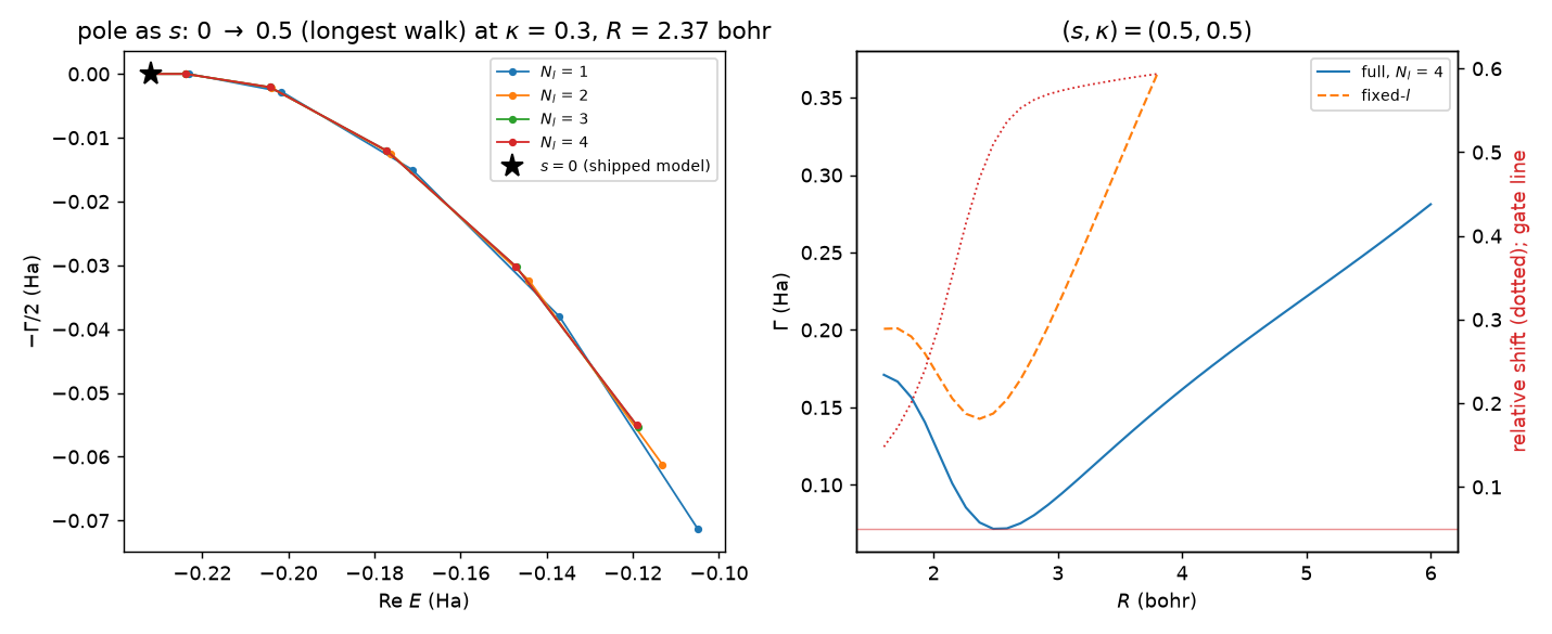
The pole in the complex plane at \(R = 2.4\) bohr as \(s\) is walked from 0 (the shipped model, star) through every channel count, at \(\kappa = 0.3\) — one pole per curve at every \(s\), the picture behind the single-pole null. The right panel’s width comparison is superseded; see below.

Physical picture

The shipped NO model represents the \(^2\Pi\) anion shape resonance as a single partial wave, \(\Lambda = 1\) (\(l = 1\)), sitting in an isotropic Gaussian well \(-\lambda(R)\,e^{-\alpha r^2}\) centred on the molecule. That is already an approximation: NO is a diatomic, not a sphere, and its true electrostatic and exchange field mixes partial waves of the same \(\Lambda\) that an isotropic well keeps decoupled.

This project makes that anisotropy explicit and geometric rather than fitted. TwoCentreWell (projects/no_coupled_channels/anisotropy.py) splits the shipped Gaussian well into two off-centre wells,

\[V_{\rm int}(\vec r, R) = -\tfrac{1+\kappa}{2}\lambda(R)\,e^{-\alpha|\vec r - d\hat z|^2} -\tfrac{1-\kappa}{2}\lambda(R)\,e^{-\alpha|\vec r + d\hat z|^2}, \qquad d = sR/2,\]

with two knobs. \(s \in [0, 1]\) moves the wells from the molecular centre (\(s=0\), where the sum collapses back to the shipped isotropic well for any \(\kappa\) — the embedding identity below) out onto the two nuclei (\(s=1\)). \(\kappa\) is the amplitude asymmetry between the two wells and is what makes the molecule heteronuclear rather than homonuclear: at \(\kappa = 0\) the well is symmetric and only even angular-momentum transfers survive, so within \(\Lambda = 1\) the resonance couples only as far as \(l = 3\); turning \(\kappa\) on opens the \(l=1 \leftrightarrow l=2\) coupling a symmetric well forbids. CoupledModel (model.py) assembles the resulting \(N_l\)-channel block Hamiltonian for \(l = \Lambda, \ldots, \Lambda + N_l - 1\) on a fixed-\(R\) electronic grid; \(N_l = 1\) is not a degenerate corner case, it is the fixed-\(l\) reduction under test, built from the same code as every coupled model so the comparison is differential.

Method

The screen. At each sampled bond length \(R\), the resonance pole of the \(N_l\)-channel electronic Hamiltonian is located exactly as the shipped model’s own poles are: two-angle ECS stability (qscat.ecs.match_angle_stable) on a coupled rather than a single-channel Hamiltonian. The screen walks a ladder of anisotropy strengths \(s = 0, 0.1, \ldots\) at fixed \(\kappa\), seeded at \(s=0\) from qscat.model.NO’s own \(v_0(R)\) (never from the approximation being measured), and stops once the narrowest point on the curve is no longer a resonance — \(\min(\Gamma/\varepsilon)\) over the points that are actually resonant reaching 1. In this campaign every walk stops by \(s = 0.5\)–\(0.6\); none reaches \(s=1\). It is repeated for \(N_l = 1, 2, 3, 4\) over \(\kappa = 0.0\)–\(0.5\), plus an \(N_l = 5\) check at \(\kappa=0.5\) for a convergence estimate, over \(R \in [1.6, 6.0]\) bohr (41 points) — the region where the resonance lives and where the crossing from bound to resonant happens as the anisotropy is turned on: at \(s=0\) only 7 of the 41 \(R\) points are resonant at all (the rest are bound, since at \(R \gtrsim 2.5\) bohr the shipped anion curve sits below the neutral one), because it is precisely the anisotropy that turns those bound points into resonances. On the \(N_l=4\), \(\kappa=0.3\) curve that count rises to 36 by \(s=0.2\) and to all 41 by \(s=0.3\) (the fixed-\(l\) and other channel-count curves reach 41 at different \(s\); this is the one the sentence above is measured on). The electronic deck used here is deliberately not the published NO deck (8 tail elements at 44°/52° rather than 6 at 35°/44°): the published deck’s tail cannot represent the resonance once the anisotropy broadens it. At \(s=0.4\), \(R=2.0\) bohr, the two-angle residual is already \(6\times 10^{-4}\) on the published deck against \(3.0\times 10^{-9}\) on this one, five orders of magnitude apart with no physics changed, and by \(s=0.5\) the published deck loses the pole outright.

The observable. A resonance curve is not itself an observable. The screen’s curve difference (coupled minus fixed-\(l\), in both \(V_d(R)\) and \(\Gamma(R)\)) is applied as a difference to the shipped qscat.core.lcp.local_complex_potential output for qscat.model.NO — linearly interpolated over the screen’s \(R\) sample and left at zero outside it, which includes the ECS complex tail. That reuses the shipped assembly’s freezing near \(R\to0\) and tail clamping untouched, so the comparison cannot manufacture a tail artefact of its own — at the price of confining the measured effect to \(R \in [1.6, 6.0]\) bohr, exactly where the screen sampled. The resulting curves ("full" and "fixed") are each run through qscat.core.lcp.lcp_ve_cross_section, the LCP’s vibrational-excitation route, over 41 energies from 0.020 to 0.100 Ha spanning NO’s resonance, for the elastic (\(v'=0\)) and first-inelastic (\(v'=1\)) channels. This is VE, never DA: NO’s dissociative-attachment channel opens at \(+0.172\) Ha, well above this sweep, so \(\sigma_{\rm DA}\) there is a \(\sim 10^{-19}\,a_0^2\) tail that the LCP is documented to miss by five to seven orders — far too poorly resolved to register a few-percent change in \(\Gamma(R)\). Because both curves are driven through the identical LCP machinery, the comparison is differential by construction: it measures the effect of the coupling, not the quality of the LCP approximation.

The shipped local_complex_potential(NO, ...) baseline both branches ride on is recomputed here on this screen’s own electronic deck (44°/52°, 8 tail elements), not on NO’s published production deck (35°/44°, 6 tail elements) — the same substitution the screen itself makes and for the same reason (see above). Measured over \(R \in [1.6, 6.0]\) bohr, the two decks’ baselines agree to \(\max|\Delta V_d| = 1.7\times10^{-4}\) Ha and \(\max|\Delta\Gamma| = 2.8\times10^{-4}\) Ha — about 0.3% of \(\max(\Gamma)\) — so the substitution is benign and does not affect any of the numbers below.

Every run also emits qscat.core.lcp.curve’s standing warning that its pole walk freezes below \(R = 1.5187\) bohr for the last 23 of 507 nuclear nodes — the small-\(R\) breakdown that module’s own docstring documents as deliberate and usually harmless. That freeze sits outside the \(R \in [1.6, 6.0]\) span this project modifies and is identical on both the “full” and “fixed” branches, so it cancels in the difference and is expected and harmless here.

The perturbation limit. The observable’s construction (the curve difference applied to the shipped LCP output, above) is only meaningful while that difference stays small relative to the curve it is added to. Measured across the campaign’s own \(s\) ladder, \(\max|\Delta\Gamma(R)|\) as a fraction of \(\max(\Gamma^{\rm shipped}(R))\) is 0.01 at \(s=0.1\), 0.62 at \(s=0.2\), 1.88 at \(s=0.3\), 2.10 at \(s=0.5\): past a fraction of about 0.2 the difference exceeds the width it is modifying, \(\Gamma^{\rm coupled}(R)\) clamps to zero across the doorway by the \(\max(0, \cdot)\) in the construction, and there is no cross section left to compare — the coupled \(\sigma_{\rm VE}\) collapses toward zero while the fixed-\(l\) one does not, and a pointwise relative-shift metric reports that collapse as if it were a 100%-or-more physical effect. The observable is therefore evaluated at the largest \(s\) where the fraction stays at or below 0.25, which on this campaign is \(s=0.1\); \(s=0.2\) already fails it.

The gate. Three criteria. (a): a genuine second pole appears anywhere in the whole campaign (read from the residual-filtered pole count, not the raw angle-stable count — a spurious near-threshold state is angle-stable at every \(R\) and every \(s\), so the raw count is 2 everywhere and cannot be the criterion). This redefinition — n_poles, not the raw angle-stable n_stable — was made before the campaign ran, so criterion (a) is exactly the pre-registered criterion. (b): the maximum relative shift in \(\Gamma(R)\) exceeds 5%, evaluated at the largest \(s\) both the fully coupled (\(N_l=4\)) and fixed-\(l\) (\(N_l=1\)) walks reached at \(\kappa=0.5\) (\(s=0.5\) in this campaign) — this criterion compares two computed curves directly, with no construction in between, so it is sound wherever both curves exist and needs no perturbation limit, and it is also exactly as specified. (c) is not: criterion (c) as originally conceived was the pointwise maximum relative shift in \(\sigma_{\rm VE}(E)\) exceeding 5% at any sampled energy. What is reported below is the median relative shift, evaluated at an \(s\) chosen by the perturbation limit above — and both of those changes were made after the first campaign run had already produced numbers, not declared ahead of it. The reason is documented in the perturbation-limit discussion just above: the pointwise-maximum form was measuring the curve-difference construction’s own collapse near and past \(s\approx0.2\), not a larger physical effect, and reading it literally would have reported that collapse as a 100%-or-more shift in the cross section. Both changes made the gate harder to open, not easier — a stricter reduction (median) and a more conservative evaluation point (\(s=0.1\) rather than whatever larger \(s\) the raw walk reached). The gate’s conclusion is unaffected by this post-hoc tightening of (c): criterion (b), which needs no construction and was never changed, opens it on its own. Because criteria (b) and (c) are evaluated at different \(s\) for two distinct reasons, they are reported with the \(s\) each used, and a reader must not assume they refer to the same point on the ladder. Any one criterion firing opens the gate; a shut gate would have been reported as prominently as the open one it turned out to be. Criteria (b) and (c) are both WITHDRAWN — see Superseded results. Criterion (b) measured a position shift rather than a width error, and criterion (c) was evaluated through the curve-difference construction on a width the unrenormalised model had already destroyed. Criterion (a), the single-pole null, stands and is now explained by the absence of any higher partial wave able to host a resonance.

Validation

At \(s=0\), every channel count from \(N_l=1\) through the \(N_l=5\) check agrees to better than \(10^{-11}\) — measured over every \(s=0\) payload in validation/coupled/results/screen.json, \(\max|\Delta V_d| = 2.79\times 10^{-12}\) Ha and \(\max|\Delta\Gamma| = 4.73\times10^{-12}\) Ha — the embedding identity built into TwoCentreWell (the two-well sum collapses to the shipped isotropic well at \(s=0\) for any \(\kappa\)) holding at full campaign scale, on the real solver rather than a toy case. That identity is what stands in for external validation once \(s>0\): no independent reference exists for this anisotropic extension, since nothing here is fit to or compared against experiment or any published curve — \(s\) and \(\kappa\) are geometric, and the anisotropic model is deliberately never treated as anything other than a testbed for the fixed-\(l\) approximation. The \(N_l=4\) vs. \(N_l=5\) channel comparison serves the same role the model has for the width claim itself: at \(s=0.3\), where the headline 58% median \(\Gamma\) discrepancy is quoted, that check agrees to 0.2%, so the discrepancy is resolved against a model that is itself two orders of magnitude tighter than the effect being reported. At \(s=0.5\) the same check is looser (2.8%), so the \(s=0.5\) number is corroboration for the \(s=0.3\) result, not the headline on its own.

Superseded results

Everything in this section was computed on the BARE two-centre well, before the normalisation requirement was understood. At \(s = 0.3\) with lam unrescaled, none of the 41 \(R\) points binds the anion, against 34 in the shipped model. Those runs therefore describe a model that has lost the state it was built to represent, and their numbers are not properties of partial-wave coupling. The measurements were real and are kept here so the record is auditable; the interpretations are withdrawn.

Withdrawn: the 58 % width discrepancy (and 59 % at \(s = 0.5\)). The measurement is faithful but compares the two truncations at DIFFERENT points on the resonance curve — 5-10 mHa apart in \(E_{\rm res}\) — and \(\Gamma\) falls steeply with \(E_{\rm res}\) (0.130 to 0.064 Ha as \(E_{\rm res}\) falls 0.112 to 0.074), so the position difference manufactures the width difference with no angular physics involved. Pinning both models to the same \(E_{\rm res}\) gives a median width difference of 0.56 % against 14.2 % unpinned, over the seven \(R\) points in \([1.6, 2.2]\) where the correctly normalised model still has a resonance:

\(R\) (bohr)	\(\Gamma\) (\(N_l{=}1\))	\(\Gamma\) (\(N_l{=}4\))	ratio	unpinned
1.6	0.103528	0.103069	0.9956	0.075
1.8	0.077123	0.076715	0.9947	0.110
2.0	0.037609	0.037387	0.9941	0.194
2.2	0.005475	0.005440	0.9936	0.423

The truncation moves the resonance POSITION; it barely touches the WIDTH. Renormalised, the two-centre model reproduces the shipped \(\Gamma(R)\) to 0.1-1.7 %, and recovers 33 bound points of 41 (34 modulo the two crossing points that do not solve) against the unrenormalised model’s 0. At \(R = 2.15\): shipped \(\Gamma = 0.011064\), renormalised 0.011244 (+1.6 %), unrenormalised 0.055500 — five times too wide.

Withdrawn: the entire bare cross-section campaign at \(s = 0.3\). It reported that the prediction of added structure was falsified (one peak per curve at two prominence floors, total variation within 1-6 %), that the peak moved a near-constant \(-16\) to \(-20\) mHa, and that the fixed-\(l\) model under-predicted the peak inelastic cross section by a factor climbing to 11.8 at \(v' = 4\). All of it describes the unbound-anion model. Renormalised, the same deck and mesh recover the shipped model’s cross section closely (\(\sigma_{\max}\) 37.101 against the control’s 37.089 at \(v' = 1\); 16.709 against 16.716 at \(v' = 2\)), with the boomerang structure present and the peak counts matching.

Withdrawn: criterion (c)’s 31 % cross-section shift at \(s = 0.1\), and the GATE OPEN verdict resting on criteria (b) and (c). Criterion (b) is the withdrawn width claim. Criterion (c) was evaluated through the curve-difference construction on the unrenormalised width. Criterion (a) — no second pole — stands, and is now explained rather than merely observed.

Withdrawn: the \(s = 0.1\) bare campaign as a source of numbers. It does recover the boomerang structure, since the anion is still bound near equilibrium, but its \(E_{\rm res}\) is displaced by 174 meV at the crossing and 343-572 meV further out, against a vibrational quantum of 239.5 meV — roughly one vibrational level, right where the Franck-Condon factors live. The qualitative observation that structure returns is sound; the peak positions and channel ratios are not quotable.

Why \(s = 0.3\) was chosen, and why that criterion was wrong. It was picked as the anisotropy at which all 41 \(R\) points are resonant, giving a complete set of comparable widths. Restated, that criterion selects the anisotropy at which the anion is nowhere bound — it required destroying the physics in order to make the comparison tidy. A separate perturbation limit in the Method section independently put the usable range at \(s \le 0.1\); both diagnostics were pointing at the same boundary.

Retained from these runs. The single-pole null, the embedding identity at \(s = 0\), the deck and mesh (validated independently: at \(s = 0\) the solver reproduces the published NO cross section on this deck, with \(v'=0\) peaking at 514 bohr² near 0.010 Ha and 9 resolved oscillations), and every piece of method documentation above.