The nonlocal resonance model (NRM)¶

Location: qscat.core.nrm (libs/qscat/qscat/core/nrm/: scattering.py, discrete_state.py, coupling.py, ingredients.py, nonlocal_potential.py, dissociation.py, vibrational_excitation.py), libs/qscat/tests/test_nrm_*.py, validation/diatomic/nrm.py + test_nrm.py and ve_nrm.py + test_ve_nrm.py + ve_nrm_figure.py, apps/qscat-run (the nrm method, tests/test_runner_nrm.py, examples/f2-da-nrm-vs-lcp-vs-exact.yaml and examples/n2-ve-nrm-vs-exact.yaml). Source: K. Houfek, T. N. Rescigno, C. W. McCurdy, Phys. Rev. A 77, 012710 (2008) — reference/literature/houfek-2008-pra77-012710.md. Every equation number below is that paper’s, with its printed-page locator. Scope: the time-independent nonlocal core and two cross sections built on it — dissociative attachment (§7) and vibrational excitation (§8). The time-dependent route is not implemented — see §11. Units: atomic units throughout (hartree, bohr).

1. What this is, and why¶

The repo already has two ends of a ladder for the 2-D electron–diatomic model:

	what it solves	role
`qscat.core.driven` / `qscat.core.dissociation`	the full 2-D driven Lippmann–Schwinger equation	the oracle
`qscat.core.lcp`	a 1-D nuclear problem on \(V_d(R) - i\Gamma(R)/2\)	an approximation, with documented failures

The local complex potential (LCP) throws away two things at once: the energy dependence of the width, and the nonlocality of the effective nuclear interaction. qscat.core.nrm restores both. It is the middle rung — still a resonance approximation, still a 1-D nuclear equation, but with a complex, energy-dependent, nonlocal kernel \(F(E,R,R')\) in place of \(-i\Gamma(R)/2\). The question it answers is how much of the LCP’s error is bought back by nonlocality alone.

The answer, measured here, has two halves. In dissociative attachment: on F₂ essentially all of it (choice B lands within 0.06–1.9 % of the exact oracle where the LCP is off by 11–74 %), and on NO, within 1.5–1.9 %, where the LCP over-predicts by 1.8e5 to 2.2e7. NO read as a total failure until 2026-08-24; that was the oracle’s error, not the model’s (§7.2). Sections 7 and 9 give both in full. In vibrational excitation, the channel the paper plots for every molecule in its study: choice B with the Eq. (37) background terms reproduces the exact 2-D solver to better than 0.7 % on N₂ and F₂, in both the elastic and the first inelastic channel — nrm-vibrational-excitation.md.

2. The method¶

2.1 The Feshbach split¶

Project onto a single “discrete state” \(\phi_d(r;R)\) and its complement. Eq. (15), (20) and (21) are on p. 012710-3; the asymptotic requirement Eq. (67) is on p. 012710-7:

\[Q = |\phi_d\rangle\langle\phi_d|, \qquad P = 1 - Q \tag{15}\]

\[V_d(R) = V_0(R) + \langle\phi_d|H_\mathrm{el}|\phi_d\rangle \tag{20}\]

\[V_{dk}^{+}(R) = \langle\phi_d|H_\mathrm{el}|\phi_k^{+}\rangle \tag{21}\]

\[\lim_{R\to\infty} \phi_d(r;R) = \phi_b(r) \tag{67}\]

\(H_\mathrm{el}\) is the electronic Hamiltonian excluding \(V_0(R)\) (Eq. 61 adds it back); \(\phi_k^{+}\) is the fixed-nuclei electron scattering function at real electron energy \(E = k^2/2\), solved in the electronic FEM-DVR-ECS basis (nrm/scattering.py). Eq. (67) is a requirement on the discrete state, not an output: as the molecule dissociates the discrete state must become the anion’s bound electronic state, at which point the discrete–continuum coupling switches off identically.

2.2 The nuclear equation and σ_DA¶

Eq. (52)-(54), p. 012710-5:

\[ \left[E - T_R - V_d(R)\right]\Psi_d^{+}(R) - \int F(E,R,R')\,\Psi_d^{+}(R')\,\mathrm{d}R' = V_{dk_i}^{+}(R)\,\chi_{v_i}(R) \tag{52} \]

\[ F(E,R,R') = \int V_{dk}^{+}(R)\,G_0^{+}(E,R,R')\,V_{dk}^{+}(R')^{*}\,k\,\mathrm{d}k \tag{53} \]

\[ \sigma_\mathrm{DA}(E) = \frac{2\pi^2}{k_i^2}\,\frac{K_\mathrm{DA}}{\mu}\, \lim_{R\to\infty}\left|\Psi_d^{+}(R)\right|^2 \tag{54} \]

dissociation.solve_nuclear assembles Eq. (52) verbatim in nuclear DVR coefficient space, \(A = E\cdot I - T_R - \mathrm{diag}(V_d) - F\), and da_sigma_from_psi evaluates Eq. (54) from the wavefunction value at the outermost real node, \(\psi[b]/\sqrt{W_b}\) — not the raw DVR coefficient. That extraction is algebraically identical to the one qscat.core.lcp.lcp_da_cross_section performs (\(\sigma = 4\pi^3|S_\mathrm{DA}|^2/2E\) with \(S_\mathrm{DA} = \sqrt{K/2\pi\mu}\,\psi(X)\) expands to \(\pi^2 K|\psi|^2/(\mu E)\), and so does Eq. (54) with \(k_i^2 = 2E\)), so the NRM and the LCP are compared on exactly the same footing.

Note the RHS: it carries \(V_{dk}^{+}\) at the incident real electron energy, evaluated directly from Eq. (21) — not the discretized \(V_{dn}\) of Eq. (59), which serves only to build \(F\) (p. 012710-6). That is why coupling.v_dk_plus exists as a separate primitive.

2.3 The ECS + DVR evaluation of F¶

Expanding Eq. (53)’s resolvent in the eigenbasis of the P-projected electronic Hamiltonian avoids the singular electron-energy integral the paper explicitly rejects (p. 012710-5):

Eq. (55) is on p. 012710-5; Eq. (56)-(61) are on p. 012710-6:

\[ F = \langle\phi_d|H_\mathrm{el} P\left[P(E - H_\mathrm{el} - T_R - V_0 + i\eta)P\right]^{-1} P H_\mathrm{el}|\phi_d\rangle_r \tag{55} \]

\[\sum_k (P H_\mathrm{el} P)_{i,k}\,\phi_n(r_k;R_j) = E_n(R_j)\,\phi_n(r_i;R_j) \tag{56}\]

\[P(R_j)_{i,k} = \delta_{i,k} - Q(R_j)_{i,k} \tag{57}\]

\[Q(R_j)_{i,k} = \sqrt{w_i}\,\phi_d(r_i;R_j)\,\phi_d(r_k;R_j)\,\sqrt{w_k} \tag{58}\]

\[ V_{dn}(R_j) \approx \sum_{i,k} \sqrt{w_i}\,\phi_d(r_i;R_j)\,H_\mathrm{el}(R_j)_{i,k}\, \phi_n(r_k;R_j)\,\sqrt{w_k} \tag{59} \]

\[ F(E,R_i,R_j) = \sum_n \sqrt{W_i}\,V_{dn}(R_i)\,M(n)^{-1}_{i,j}\,V_{dn}(R_j)\,\sqrt{W_j} \tag{60} \]

\[M(n)_{i,j} = \left[E - T_R - V_0(R) - E_n(R)\right]_{i,j} \tag{61}\]

\(w_i\) are the electronic DVR weights, \(W_i\) the nuclear ones. Four attached conditions are load-bearing, all on p. 012710-6:

No conjugation. \(P H_\mathrm{el} P\) under ECS “is symmetric, but not Hermitian, [so] we have to use for the wave functions \(\phi_n(r;R)\) the scalar product defined without complex conjugation”. ingredients.py contracts bilinearly throughout (qscat.linalg.c_product, a plain np.dot). Note Eq. (60) carries \(V_{dn}(R_j)\), not \(V_{dn}(R_j)^{*}\), even though the undiscretized Eq. (53) it evaluates is written with \(V_{dk}^{+}(R')^{*}\).
\(E_n\) is R-dependent. Eq. (56) is solved at every nuclear node, and Eq. (61) carries \(E_n(R)\) inside the nuclear matrix. nonlocal_operator passes a per-node vector into np.diag; nothing is frozen. (\(E_n\) is frozen only in the ECS tail — see §5.)
No regulator. “We have avoided singularities in constructing the inverse of \(M(n)\) since the energies \(E_n(R)\) are complex whereas the total energy \(E\) of the system is always real.” Eq. (55)’s \(i\eta\) is not carried into the discretized form. Measured conditioning: the worst min |eig M(n)| over all 131 states and E = 0.005 / 0.05 / 0.20 Ha is 4.3e-3, max cond(M) = 4.3e4. The floor is set by the lowest ECS continuum state’s |Im E_n|, which scales as ~1/r_max² of the electronic box — bounded and predictable, not a cliff.
The state sum runs over \(N - 1\) states. \(P = 1 - |\phi_d\rangle\langle\phi_d|\) has an exact zero mode whose eigenvector is \(\phi_d\) itself (\(P\phi_d = 0\)), a Q-space direction rather than a P-space one. ingredients._drop_null_mode identifies it by two criteria and raises rather than guessing (measured margin: min|E_n| = 6.2e-3 against a null |E| ~ 1e-10, null-mode overlap 1.0 with next-largest 3.7e-11).

The \(\sqrt{W}\) factors of Eq. (60) are not applied, and that is correct. Eq. (58) and (59) fix the paper’s own convention — \(\sqrt{\text{weight}} \times \text{function value} = \text{DVR coefficient}\), operator matrices coefficient-space — and Eq. (61) says \(M(n)\) is the nuclear operator “in this representation”. Under that reading the coefficient-space matrix of \(F\) is \(\sum_n V_{dn}(R_i)\,M(n)^{-1}_{i,j}\,V_{dn}(R_j)\) with no surviving \(\sqrt{W}\): the two factors that convert \(\Psi_d\) to and from coefficients are the ones already inside \(M(n)^{-1}\). Eq. (60) as printed is self-consistent only if its \(M(n)^{-1}_{i,j}\) means the function-space Green’s kernel value rather than the inverse of the coefficient-space matrix Eq. (61) defines; the paper does not resolve the ambiguity. The local limit settles it: neglecting \(T_R\) makes the code’s expression collapse to \(\mathrm{diag}\left(\sum_n V_{dn}^2/(E - V_0 - E_n)\right)\), whose imaginary part is \(-(i/2)\Gamma(E,R)\) — a diagonal potential in coefficient space, which is what a DVR local potential looks like. With the extra \(\sqrt{W_i}\sqrt{W_j}\) it would be \(\mathrm{diag}(W_i \cdot \ldots)\), which is not a potential.

2.4 The width and the cutoff¶

Eq. (68)-(69), p. 012710-8:

\[\Gamma(E,R) = 2\pi\,|V_{dk}^{+}(R)|^2, \qquad E = k^2/2 \tag{68}\]

\[f(r) = 1 - \frac{1}{1 + e^{-(r - r_d)}}, \qquad r_d = 10\,a_0 \tag{69}\]

Eq. (69)’s smooth cutoff applies only to the scattering-derived discrete state (choice A). A bound state is already square-integrable, and truncating it destroys the exact eigenrelation \(H_\mathrm{el}(\infty)\phi_b = E_b\phi_b\) on which Eq. (67)’s decoupling rests: the identity \(V_{dk} = E_b\langle\phi_b|\phi_k^{+}\rangle = 0\) holds because of P-space orthogonality. Applying the cutoff to the bound branches was a real defect during development — it left \(|V_{dk}|\) on a spurious plateau of 2.47e-3 for every \(R \geq 5\) (identical to eight digits), i.e. a nonzero \(\Gamma(R\to\infty)\) ≈ 3.8e-5 Ha exceeding the physical width everywhere beyond R ≈ 2.6. With the cutoff restricted to the scattering branch, \(|V_{dk}|\) at R = 5 / 9 / 14 / 20 drops from 2.481e-3 / 2.466e-3 / 2.466e-3 / 2.466e-3 to 1.801e-5 / 3.390e-5 / 3.390e-5 / 3.390e-5, a factor ~73. The residual floor is understood to seven digits: the identity \(V_{dk}(R\to\infty) = (E_b/E)\cdot d\cdot(E - H_\mathrm{free})J_k\) predicts 3.389800e-05 against an actual 3.389800e-05. It is scattering.py’s ECS-masked incident wave, and it scales away with the electronic box (1.40e-5 / 4.4e-6 / 6.5e-8 / 2.5e-11 at r_max = 16 / 24 / 32 / 48), giving a \(\Gamma\) floor of ~1.2e-9 Ha — three orders below the repo’s documented 1e-6 width floor, i.e. negligible.

3. The two discrete-state choices¶

The paper’s headline methodological point is that the nonlocal model is completely determined by \(\phi_d\), and that different reasonable choices give materially different answers (Sec. VI). Two of its three are implemented, behind one DiscreteState protocol; both return DVR coefficients \(d_i = \sqrt{w_i}\,\phi_d(r_i)\), c-normalized to 1, so Eq. (58)’s projector is literally outer(d, d) with no further weights and the c-normalization already supplies the paper’s phase-fixing \(e^{-i\delta(R)}\) (p. 012710-8) — up to the residual \(\pm 1\) that §5 has to fix by hand for the P-space states \(\phi_n\), since c_product(d,d) = 1 admits both d and −d.

That residual is harmless here, for two reasons rather than by assumption. \(Q = \mathrm{outer}(d,d)\) and \(V_d = d\cdot H_\mathrm{el}\cdot d\) are quadratic in \(d\), so a per-node sign cancels outright. \(V_{dn} = d\cdot H_\mathrm{el}\cdot\phi_n\) is not — it is linear in \(d\), and Eq. (60) contracts it at two different \(R\) — but the only branch on which \(\phi_d\)’s sign is arbitrary (the bound one, whose eigenvector comes from np.linalg.eig) is exactly the branch where \(V_{dn} \equiv 0\). Measured for choice A on F₂’s production deck: max |V_dn| is 6.1e-12 on the 572 bound nodes against 0.543 on the 247 scattering ones, and \(\phi_d\) in fact never flips — all 818 adjacent-node overlaps c_product of \(\phi_d(R_j)\) with \(\phi_d(R_{j+1})\) are positive, minimum 0.985. Choice B stores one vector, so the question does not arise for it at all.

Choice A — PhysicalDiscreteState (Sec. VI A, p. 012710-7–8). The “intuitive” one: at each R, the fixed-nuclei electron scattering function at the real part of the ECS resonance energy, smoothly truncated by Eq. (69). Where the anion is genuinely bound the pole walk reports a negative shift and the state is the bound eigenvector instead, used raw. This is exactly the quantity qscat.core.lcp.resonance_pole_walk computes and qscat.core.lcp uses directly as its \(V_d\)/\(\Gamma\) curve — so choice A is the nonlocal model’s counterpart of the LCP’s own discrete state.

Choice B — AsymptoticDiscreteState (Sec. VI B, p. 012710-9). The \(R \to \infty\) bound state \(\phi_b\), used at every \(R\). One electronic eigenproblem for the whole calculation; Eq. (67) holds trivially. R_inf is a nuclear coordinate — the outermost real node of the nuclear deck (F₂ 10.7, NO 9.0 bohr), never the electronic grid’s ECS radius, or \(\phi_d\) is not an \(H_\mathrm{el}\) eigenvector there and the tail-coupling guard rejects the ingredient set. \(\phi_b\) is verifiably asymptotic at that radius: its c-product overlap with \(\phi_b\) at R_inf = 30 is 1.00000000 and \(E_b\) is stable to 1e-7 relative from 14 to 30 bohr.

Choice C, the paper’s “compact” tuned state (Sec. VI C, Eq. 70–72), is not implemented — its \(\lambda_d(R)\) are model-specific tuning functions used to demonstrate sensitivity, not physical constants.

3.1 The two choices genuinely differ, and choice A’s kernel has a step¶

At F₂’s bound/resonant crossing R_c ≈ 2.59 bohr, choice A’s max |V_dn| jumps from 2.9e-12 to 2.64e-1 across a single \(\Delta R = 0.02\) step (R 2.60 → 2.58, measured after _sign_align landed): on one side \(\phi_d\) is a bound eigenvector (so \(V_{dn} \equiv 0\) by orthogonality), on the other it is an Eq. (69)-truncated scattering function. Eq. (60) is bilinear in \(V_{dn}(R_i)\,V_{dn}(R_j)\), so choice A’s \(F\) kernel is discontinuous in \(R\). The paper’s \(e^{-i\delta(R)}\) phase-fixing exists to make \(\phi_d\) vary smoothly across the crossing and cannot remove this step. Choice B is smooth over the same span (state n = 3: 1.2e-7 at R = 6 rising monotonically to 2.2e-2 at R = 1.8, no flips).

That \(V_{dn} \equiv 0\) on a bound branch is not a convenience — it is what the paper demands (p. 012710-7: “Because the bound state is the eigenfunction of \(H_\mathrm{el}\), the discrete-state–continuum coupling \(V_{dk}(R)\) goes to zero … a nonzero coupling even for very large internuclear distances … has no physical meaning”). It is Eq. (67) satisfied exactly rather than asymptotically, and it is a general algebraic consequence, independent of grid, molecule and ECS leakage. \(F \equiv 0\) wherever either argument is on the bound branch is likewise intended: no open continuum means no autodetachment, and the DA exit channel propagates on the real \(V_d(R)\).

4. Naming: PRA 77’s V_d is not qscat’s LCP `Vd`¶

A genuine collision, and worth stating plainly because both appear in this repo:

symbol	meaning	qscat name
PRA 77’s \(V_d(R)\), Eq. (20)	the discrete-state potential \(V_0(R) + \langle\phi_d\vert H_\mathrm{el}\vert\phi_d\rangle\)	`NrmIngredients.v_d_discrete`
paper I’s / PRA 77’s \(E_\mathrm{res}(R)\)	the real part of the fixed-\(R\) ECS resonance pole	`qscat.core.lcp`’s `Vd`, and `docs/physics/lcp-resonance-levels.md`’s `E_res(R)`

The paper states the two “almost coincide” for the physical discrete state (p. 012710-8) — not that they are identical, and not for choice B. Measured at each molecule’s doorway peak, |V_d(B) − V_d(LCP)| is 0.0053 Ha for F₂ and 0.0229 Ha for NO. Anything that reads one for the other is wrong by that much.

How much that is, on an observable. Gertitschke & Domcke, Phys. Rev. A 47, 1031 (1993) Eq. (2.15) propagates \(T_N + V_d + \Delta_L - (i/2)\Gamma_L\), and its Eq. (2.14) fixes which of the two goes in: \(V_d + \Delta_L = E_\mathrm{res} + V_0\), i.e. the LCP Vd, with v_d_discrete short by the level shift \(\Delta_L\). Substituting v_d_discrete there anyway and running the resulting propagation against lcp_da_cross_section on one F₂ deck gives \(\sigma/\sigma_\mathrm{LCP}\) = 0.346 / 0.419 / 7.14 at E = 0.02 / 0.03 / 0.05 Ha, against 1.000215 / 1.000198 / 0.999892 for the correct reading — so the confusion is worth orders, not percent, and it changes direction with energy. Details and the \(\Gamma\)-supported V_d difference profile: docs/physics/nrm-time-dependent.md §6.1.

5. What the implementation adds that the paper does not describe¶

Two things, both necessary, and they are where a molecule-specific corruption could hide:

Adiabatic labelling (ingredients._track, _sign_align). Eq. (60)–(61) require the label \(n\) to mean the same P-space state at \(R_i\) and \(R_j\) — \(M(n)\) is built from the curve \(E_n(R)\), and \(F\) contracts \(V_{dn}(R_i)\) with \(V_{dn}(R_j)\) for one \(n\). The paper never says how \(n\) is assigned across \(R\). _track does greedy nearest-eigenvalue matching; _sign_align then orients each eigenvector against its predecessor by sign(Re c_product), which is necessary because np.linalg.eig returns an arbitrary phase per node and c-normalization fixes the scale only up to \(\pm 1\) (for a complex-symmetric matrix under the bilinear c-product, \(c^2 = 1 \implies c = \pm 1\), per nondegenerate eigenvalue). Without it, measured sign flips at |V_dn| ~ 0.1 — against a spectrum maximum of 0.19 — flipped individual (n,i,j) contributions to \(F\), producing a wrong-but-plausible kernel. Verified clean on the production decks for choice B: min |c_product(prev,cur)| = 0.99998709 (NO) and 0.99629559 (F₂), zero pairs below 0.5, max relative E_n jump ~1e-3. (Provenance: unlike most numbers in this note, that pair is a single-run measurement — it costs ~15 min and ~14 GB, so it was not independently re-run. It is the one load-bearing datum behind “the choice-B collapse is not a tracking artifact”; anyone re-opening §9 should re-measure it first.)

ECS-tail continuation (nonlocal_potential.continue_to_tail). Ingredients are built on the nuclear grid’s real nodes only, and the complex-scaled tail is filled with the outermost real value. Eq. (56) is stated for every nuclear node including the complex ones, so this is a substitution — but a benign one, because \(\lambda(R) = \lambda_\infty + \lambda_0/(1 + e^{\lambda_1(R - R_\lambda)})\) has saturated long before the ECS pivot (NO: e^{−49.6} from its limit at R = 12; F₂: e^{−32.7}), making \(H_\mathrm{el}(R)\) R-independent to machine precision across the whole tail. \(V_0(R)\) — the part that matters for the outgoing boundary condition — is evaluated on the complex contour in nonlocal_operator’s own v0 term. dissociation.nrm_da_cross_section’s v_d_full is the one exception: it freezes the WHOLE discrete-state potential \(V_d(R) = V_0(R) + \langle d|H_\mathrm{el}|d\rangle\) (Eq. 20) at its outermost-real value across the tail via continue_to_tail, the opposite convention from the sibling qscat.core.lcp (which freezes only the electronic shift and evaluates v0 itself on the contour). Measured harmless: |v0(tail) − v0(R0)| ≤ 6.5e-7 Ha (F₂) and ≤ 1.1e-5 Ha (NO) across every tail node, against exit energies of 0.077 and 0.0031 Ha.

5.1 What `TAIL_COUPLING_MAX` actually catches¶

Key result: shrinking the ECS pivot does not walk check_tail_coupling toward tripping — the guard is flat against genuine ingredient sets and fires only on a structurally malformed one, six orders of magnitude away.

For AsymptoticDiscreteState built at R_inf = R0 (the production choice), \(\phi_d\) is by construction an exact eigenvector of \(H_\mathrm{el}(R_0)\), so \(V_{dn}(R_0)\) is zero identically regardless of how large or small the box is. Measured on F₂/NO: max |V_dn(R0)| is 1.8e-12 at R0 = 6.0 and 2.4e-12 at R0 = 10.7 for F₂, and 6.8e-13 at R0 = 6.0 and 1.0e-12 at R0 = 10.7 for NO — order \(10^{-13}\)–\(10^{-12}\) Ha across every case tried, and flat in R0. What the guard actually catches is a truncated or otherwise malformed ingredient set — one whose outermost node is not genuinely \(\phi_d\)’s R_inf (e.g. \(\phi_d\) pinned at R_inf = 10.7 but the ingredient range only sampled out to R = 6.0): measured 7.2e-7 there, within a factor of ~1.4 of TAIL_COUPLING_MAX = 1e-6 and ~\(10^6\) times the genuine R0 values above.

6. Validation¶

Four independent checks, none of which is a restatement of the code’s own formula.

(a) The \(\Gamma\) gate — Eq. (68) against the LCP’s independent pole width. \(\Gamma = 2\pi|V_{dk}^{+}|^2\) must reproduce the width qscat.core.lcp gets from two-angle ECS pole matching, a completely different computation. On F₂, in a window where the comparison is meaningful (\(\Gamma/E < 0.35\), \(E_\mathrm{res} > 0.02\) Ha, 14 points), the median ratio is 1.013, range [0.974, 1.044], max deviation 0.0439. The gate discriminates: injected mutations \(V \to V/\sqrt{2}\) (0.513), \(V \to V/2\) (0.756), \(V \to 2V\) (3.18) and writing \(\pi\) for \(2\pi\) in Eq. (68) (0.513) all fail it.

The residual is understood and is not an error. \(\Gamma_\mathrm{LCP}\) is the width at the complex pole, while Eq. (68) evaluates the coupling at the real resonance energy. With \(\Gamma \sim E^{3/2}\) near threshold, \(|\Gamma(E-i\Gamma/2)/\Gamma(E)| \approx \sqrt{1 + (0.75\,\Gamma/E)^2}\), which predicts the observed trend: the ratio passes through 1.0023 at \(\Gamma/E = 0.30\) and drifts to 0.72 by \(\Gamma/E \approx 1.33\), F₂’s broad-resonance end. Supporting evidence that the coupling itself is right: grid-converged to three decimals over r_max 16→24→32, order 8→10, n_complex 6→10; the Wigner exponent \(\mathrm{d}\ln\Gamma/\mathrm{d}\ln E \to 1.45\) against the expected \(l + \tfrac12 = 1.5\); and dropping the projector \(P\) makes \(\Gamma\) 46× larger, so \(P\) is load-bearing.

Two limits, stated because they matter downstream. The gate compares \(|V|^2\) only, so the phase of \(V_{dk}^{+}\) is ungated by it. And on NO the window is empty — 47 genuinely-tracked open points, 0 inside. The reason is sharper than “NO’s resonance is broad everywhere”: its \(\min\,\Gamma/E\) on the tracked branch is 0.124, comfortably inside the 0.35 cut. The two cuts simply never overlap. \(\Gamma/E\) rises monotonically inward and crosses 0.35 at \(R \approx 2.196\), where \(E_\mathrm{res}\) is still 0.0158 Ha; the last narrow point (\(\Gamma/E = 0.338\) at \(E_\mathrm{res} = 0.0150\)) is below the gate’s 0.02 Ha energy floor, and the first point above the floor is already broad (0.409 at \(E_\mathrm{res} = 0.0202\)). NO’s resonance is narrow only where it is also near threshold. So on NO the coupling carries only an order-of-magnitude cross-check.

(b) The local limit of \(F\). With \(\mu \to \infty\), \(T_R \to 0\) and Eq. (60) must collapse to the analytic second-order level shift \(F_{ij} = \delta_{ij}\sum_n V_{dn}^2/(E - V_0 - E_n)\). Measured relative error: 5.6e-1 at physical \(\mu\), then 2.4e-6 / 2.4e-9 / 2.4e-12 at 1e6 / 1e9 / 1e12 × \(\mu\) — clean \(1/\mu\) convergence, with the off-diagonal part vanishing at the same rate. This pins the assembly, the \(E\cdot I - T_R - V_0 - E_n\) sign convention and the weights (the nuclear grid weights span 0.0074–0.74, so a double-apply would show as a 1e-2…1 factor). Im diag F ∈ [−2.8e-3, 0] — the correct \(-i\Gamma/2\) absorption sign. Separately, \(F\) is complex-symmetric and genuinely nonlocal: |F − Fᵀ|/|F| = 1e-16 against |F − F†|/|F| = 0.17, with off-diagonal/diagonal magnitude 0.17.

(c) The LCP local-limit bridge. Driving solve_nuclear with \(F \to \mathrm{diag}(-(i/2)\Gamma)\) and the LCP’s own doorway must reproduce lcp_da_cross_section — already-validated code, used as a differential oracle. It does, to 2.7e-14 relative on F₂ (0.034104733597583474 against 0.0341047335975844) and 2.3e-14 on NO’s own deck. The bridge gates the operator assembly, the \(F\) application, and the whole flux extraction (boundary node, weight, prefactor, threshold): mutating the boundary to the outermost grid node gives 7e-59, to the second-outermost real node 0.9984, dropping \(\sqrt{w_b}\) 3.6e-3, doubling \(1/w_b\) 281. Flipping \(-F\) to \(+F\) gives only 1.0109 here — the local \(F\) is weakly absorbing, so the bridge catches that sign by just 1.1 %; with the true nonlocal \(F\) the same flip moves \(\sigma\) by 3.13×. It does not gate nrm_da_cross_section’s own wiring — the energy bookkeeping and the \(F\)/coupling calls — which is covered separately by an assertion that \(F\) moves \(\sigma\) by >2× at E = 0.03 (measured 5.152×; do not move that test to a cheaper energy, \(F\) shifts \(\sigma\) by only ~12 % at E = 0.02).

(d) σ_DA against the exact 2-D oracle. §7.

6.2 The Eq. (60) state sum: where to truncate, and what it looks like¶

n_states = 100 is a measured value, not a preset. The ladder (F₂, choice B, E = 0.03 Ha, σ in bohr²) was run on the 584-node development deck, not §7’s 974-node production one — so its σ values are not comparable to §7.1’s 1.65514 at the same molecule, choice and energy. What transfers is the shape of the convergence, which is what the ladder is for:

n=  10  0.01751     n=  70  0.03773  (1.97 % from full)
n=  25  0.01566     n=  75  0.03838  (0.27 %)
n=  50  0.02565     n=  80  0.03848  (0.008 %)
n=  65  0.03572     n= 100  0.038485976993408715
                    full (131) 0.038485976993410095   (3.6e-14)

Two things this shows. First, the contribution is not front-loaded: a naive 25→50→100 doubling does not converge (50→100 is 33 % apart), and the 1 % level is not crossed until n ≈ 73–74. Second, the summand is sparse and alternating, not a smooth band. States alternate between near-zero \(V_{dn}\) (1e-11…1e-15 — deeply ECS-rotated states with large negative \(\mathrm{Im}\,E_n\), nearly decoupled from \(\phi_d\)) and \(O(0.1\text{--}0.5)\) states with small, nearly real \(E_n\). The contributing states’ \(E_n(R=2.5)\) at n = 50, 55, 60, 65, 75 are 5.9, 7.3, 11.0, 15.2, 32.3 Ha — a spread, not one resonance energy — with the marginal contribution shrinking as \(E_n\) grows through Eq. (61)’s energy denominator. The right description is “the coupling-weighted density of P-space states near the real axis, falling off with electron energy”, not “the states near the resonance”.

The convergence shape is molecule-dependent and was not predictable a priori. NO, choice B, at E = 0.20 Ha overshoots the converged value by ~217× at n = 10 (1.28e-9 against 5.92e-12) before settling by n ≈ 65–70 — the opposite of F₂’s monotone undershoot. All four molecule × choice combinations reproduce the untruncated 131-state sum to numerical identity at n = 100 (these four were measured on the production decks):

combo	<1 % at	plateau (<1e-6 rel)	identical to full
F₂ / B	75	80	95
F₂ / A	40	55	90
NO / B	70	70	100
NO / A (not converged, see §11)	40	55	90

Choice A converges faster on both molecules, consistent with \(V_{dn} \equiv 0\) on its bound branch — measured, not deduced from it.

7. Measured results — dissociative attachment¶

All numbers below are on each molecule’s own eMoScat production deck: electronic r_max = 16, order = 8, n_complex = 6 (n = 132) × the fine per-molecule nuclear deck (F₂ n = 974 with 819 real nodes; NO n = 597 with 507). v_init = 0, n_states = 100, SuperLU backend. The exact 2-D da_cross_section is the oracle; the LCP and both NRM choices are the approximations under test.

7.1 F₂ — the nonlocal model reproduces the oracle¶

F₂’s DA channel is exothermic (threshold −0.0691 Ha), so it is open at every positive E.

E (Ha)	σ exact	σ LCP	σ NRM-A	σ NRM-B	LCP/ex	A/ex	B/ex
0.010	5.36634	1.41038	1.56835	5.46688	0.263	0.292	1.0187
0.020	3.35886	1.56292	2.25416	3.36989	0.465	0.671	1.0033
0.030	1.65611	1.47242	1.39751	1.65514	0.889	0.844	0.99941
0.040	0.71510	1.01869	0.61046	0.71415	1.425	0.854	0.99867
0.050	0.28238	0.48945	0.25431	0.28211	1.733	0.901	0.99903

F₂ σ_DA: exact vs LCP vs NRM(A) vs NRM(B)

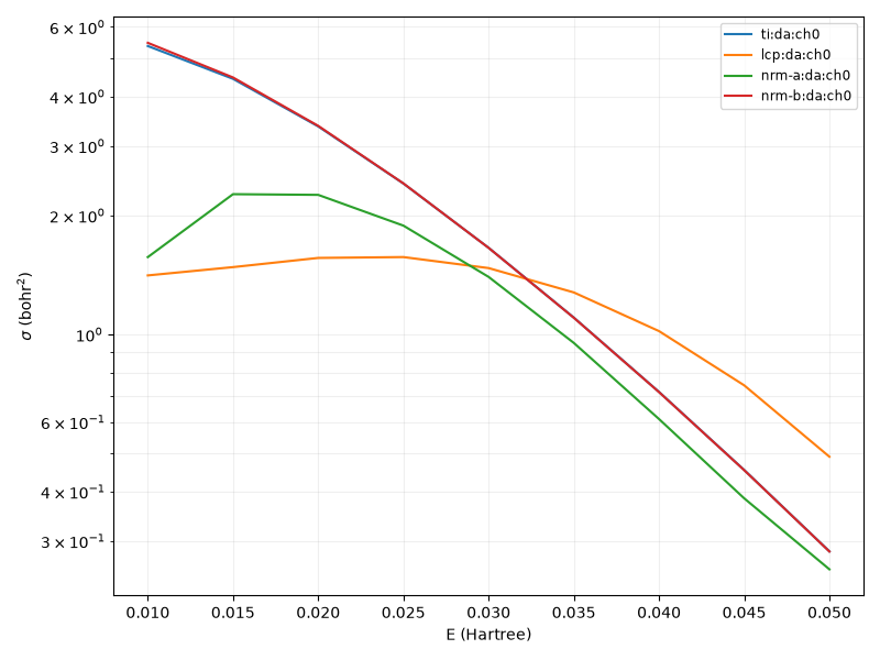
The figure is the same comparison on a nine-energy grid (0.010…0.050 Ha, step 0.005), produced in one qscat-run run from apps/qscat-run/examples/f2-da-nrm-vs-lcp-vs-exact.yaml (§12), which also writes the underlying cross_section.csv/.npz (gitignored, like every other figure’s data in this repo — rerun the config to regenerate). The exact and choice-B curves are visually indistinguishable, the LCP crosses the exact near E ≈ 0.032, and choice A sits below the exact everywhere (above the LCP below E ≈ 0.028, below it above). That run’s ti and nrm-* values reproduce the table above digit for digit; its lcp values differ by 0.05–0.15 % because qscat-run runs the pole walk at its own settings (electronic ECS angles 35°/44°, re/im_half_width = 0.01) rather than validation/diatomic/nrm.py’s 35°/40° and library defaults. That is far below the LCP’s own 11–74 % error and changes nothing here.

Choice B beats the LCP at every anchor, by factors 39 / 163 / 189 / 319 / 758. Its deviations from the oracle are

E (Ha)	0.010	0.020	0.030	0.040	0.050
\|σ_B/σ_exact − 1\|	1.9 %	0.33 %	0.059 %	0.13 %	0.097 %
× the oracle’s own floor	340	61	11	25	18

The oracle’s floor is measurable in-repo: an independent 1000-point resonance-aware grid gives \(\sigma_\mathrm{DA}\)(F₂, 0.03) = 1.6562 against this 974-point deck’s 1.65611 (docs/physics/discretisation-tuning.md:193, validation/tuning/test_resonance_aware.py), i.e. 5.4e-5 relative. Every deviation above is 11–340× that, so all of them are physics rather than grid noise and a specific figure is defensible: choice B reproduces the exact 2-D σ_DA to 0.06–0.33 % at four of the five anchors and to 1.9 % at the lowest (E = 0.010, the one nearest threshold). The sub-0.1 % entries are quoted to one significant figure — they are only ~10× the floor. The rise toward threshold is resolved, monotone below E = 0.030, and is the physically interesting part rather than an error bar.

Choice A is the degraded one, exactly as PRA 77 Sec. VI A predicts. It under-predicts systematically and worsens toward threshold (0.901 → 0.292), sitting 38–266× further from the oracle than choice B at every anchor. This is the Born-Oppenheimer breakdown the paper documents for DA (p. 012710-9, Fig. 6) — on F₂, the only molecule for which that paper publishes a DA cross section at all (§7.2) — reproduced here independently. Note choice A does not beat the LCP everywhere: the LCP is closer at E = 0.030.

The LCP’s own error, for contrast, is systematic and energy-dependent, not a fixed percentage: the ratio sweeps 0.263 → 1.733 across this window, crossing unity near E ≈ 0.032 (see docs/physics/diatomic-ve-cross-sections.md). Nonlocality is what removes that sign change.

7.2 NO — the nonlocal model was right, and the oracle was wrong¶

NO’s DA channel opens at +0.1719 Ha, so the anchors sit just above it.

This section previously recorded an unexplained collapse of choice B by 5–8 orders. That collapse does not exist. It was the exact 2-D oracle’s own error, charged to the model. Corrected 2026-08-24; the history is kept below because the way it hid is more instructive than the numbers.

E (Ha)	σ exact	σ LCP	σ NRM-A (not converged)	σ NRM-B	LCP/ex	B/ex
0.175	7.429e-10	1.30498e-4	1.03427e-3	7.540e-10	1.76e5	1.0152
0.180	2.789e-10	1.32975e-4	8.94472e-4	2.833e-10	4.77e5	1.0157
0.185	1.052e-10	1.35174e-4	7.44567e-4	1.069e-10	1.28e6	1.0165
0.190	3.986e-11	1.34727e-4	6.07468e-4	4.055e-11	3.38e6	1.0173
0.200	5.810e-12	1.29558e-4	4.19477e-4	5.921e-12	2.23e7	1.0191

Choice B reproduces the exact NO σ_DA to 1.5–1.9 % — the same quality it already has on F₂ (§7.1) — and its swing across the anchors (127.3) matches the exact swing (127.9) to 0.5 %. The LCP over-predicts by 1.8e5 → 2.2e7 and choice A by 1.4e6 → 7.2e7, both flat against a curve that falls two orders. That is the Born–Oppenheimer breakdown PRA 77’s Sec. VI A predicts, previously buried under an oracle error.

The NRM-A column is still not converged and must not be quoted as a property of choice A — see §11. Its ingredient set is corrupted at the nuclear node carrying the largest \(|\chi_0|\) on the grid.

7.2.1 The defect, because the mechanism generalizes¶

da_cross_section extracted σ from the post-form volume T-matrix \(\langle \phi_e F_K | V_{DR} | \Psi^{+}\rangle\). That is formally exact, but \(V_{DR} = V_\mathrm{int}(r,R) + v_0(R) - V_\mathrm{int}(r,R_\infty)\) does not decay in \(r\). The integrand’s size is set by the interaction region while σ_DA is set by how completely that region cancels, so the required cancellation is integrand / answer: ×2.7 on F₂ (σ ~ 1 \(a_0^2\)) and ×1.5×10⁶ on NO (σ ~ 1e-9 \(a_0^2\)). At that depth every box edge leaks, and two did — the electronic extent r_max = 16 bohr (eMoScat’s own NO deck runs the electronic real region to 90 bohr) and the nuclear R_inf = 9.0, where NO’s Morse \(v_0\) is still −1.0e-5 Ha against a true \(|T|\) of 1.4e-6.

That is why fixing one edge was not enough: r_max 16→64 moved σ(0.175) from 1.61e-2 to 5.78e-7, and R_inf 9→15 then moved it to 7.43e-10. A ladder in one parameter looked converged while the other was wide open.

The fix reads the outgoing flux instead — the extraction lcp_da_cross_section has always used — applied to the exact \(\Psi^{+}\): \(\psi_n(R) = \langle\phi_e|\Psi^{+}\rangle_r\), \(S = \sqrt{K/2\pi\mu}\,\psi_n(X)\) at the outermost real nuclear node, \(\sigma = 4\pi^3|S|^2/2E\). No cancellation, hence no edge sensitivity: invariant to 4 digits over r_max 16→96, 6 digits over R_inf 9→15, 7 digits over DVR order 8→12, and identical under SuperLU and MUMPS.

7.2.2 Why it survived an equation-by-equation audit¶

Every check ran against the approximation. The oracle was the fixed point of the comparison and was never itself compared to anything — and on F₂, where the required cancellation is only ×2.7, it was right, which made the shared code look validated.

Four things would each have caught it, and all four were cheap:

Run both extractions where both exist. Flux and volume agree to 5e-4 on F₂ at every energy and at r_max 16/32/64. One such comparison on NO would have found this in minutes.
Ladder every box parameter, not one. A plateau in r_max was mistaken for convergence while R_inf was untested.
Compare the required cancellation to the answer. ×1.5e6 is a warning in itself; no formally-exact expression survives that numerically by luck.
Read the sources for what they contain, not for what a note extracted. The campaign concluded no published NO DA reference existed, on the strength of PRA 77’s panel inventory. Váňa 2017 Fig. 3.14 (p. 46) had one all along — and its axis annotation, an LCP curve drawn ×10⁻⁵, states LCP/exact ≈ 1e5 as a datum. The old code gave 8.1e-3; the corrected code gives 1.757e5.

validation/diatomic/test_nrm.py now gates NO σ_DA against that figure, and the old flatness assertion — which encoded the oracle’s error as a requirement — is gone.

This does not contradict PRA 77. The paper contains no NO or N₂ dissociative- attachment cross section at all, for any discrete-state choice. Its two DA panels — one in Fig. 6 (p. 012710-9), one in Fig. 8 (p. 012710-10) — are F₂ panels; every other panel of Figs. 4–6 and 8 is vibrational excitation. The reason is arithmetic:

	DA threshold	windows the paper plots
N₂	+0.5016 Ha	0.05–0.17, 0.08–0.20 Ha
NO	+0.1719 Ha	0.01–0.08 Ha
F₂	−0.0691 Ha (open at any \(E > 0\))	0.00–0.10 Ha

NO’s channel opens at more than twice the top of every NO window plotted; N₂’s at about 2.5×. Both are energetically shut throughout everything PRA 77 published, so Sec. VI B’s “gives exact results” sentence for DA rests on the single F₂ panel. The NO run here is an extension beyond the paper’s tested range, at more than twice the highest energy the paper studied for NO — not a comparison against it. The reference note reference/literature/houfek-2008-pra77-012710.md was corrected for exactly this over-generalization and now carries the panel inventory and the threshold table; the claim that PRA 77 demonstrates exact DA “in all three molecules” is the false premise that drove a substantial part of this investigation in the wrong direction.

8. Vibrational excitation¶

Moved to its own note: nrm-vibrational-excitation.md — the Eq. (28)/(31)/(37)/(38) two-potential decomposition, the φ⁻ gate, the VE state sum, the figure, and the measured result: choice B + background reproduces the exact driven.ve_cross_section oracle to better than 0.7% on both N₂ and F₂ (worst ratio 0.99623–1.00692 over all four molecule/transition pairs), while choice A degrades to 0.565–1.140. That note’s §1–§10 are this section’s former §8.1–§8.10; the sections below keep their original numbers (§9–§13) so existing references to them — including qscat.core.nrm.ingredients’s “Sec. 5 and Sec. 11” — stay valid.

9. What was not explained, and what it turned out to be¶

Resolved 2026-08-24. This section recorded choice B’s five-to-eight-order collapse on NO as unresolved — no located defect, no confirmed mechanism — after an equation-by-equation audit against Eq. (55)–(61), eight killed hypotheses and two killed mechanisms. All of that work was sound and none of it could have succeeded, because the defect was not in the model. It was in the oracle (§7.2.1): a post-form volume T-matrix whose required cancellation is integrand/answer, ×1.5e6 on NO, so every box edge leaked. Choice B was within 1.5–1.9 % of the truth the whole time.

The ruled-out list below is retained because it remains correct, and it is what makes the conclusion airtight in hindsight: the model’s ingredients, doorway, coupling convention and T-matrix machinery were all verified sound — exactly what one would expect of a model being blamed for someone else’s error.

The methodological lesson, which is the part that generalizes. Every check ran against the approximation. The oracle was the fixed point of the comparison and was never itself compared to anything. §7.2.2 lists the four cheap checks that would each have caught it.

What was ruled out, all of it still valid:

An equation-level defect. An equation-by-equation audit against Eq. (55)–(61) found none: \(E_n\) is R-dependent as required, the \(\sqrt{W}\) omission is correct (§2.3), the c-product form is the paper’s own, and Eq. (52)/(54)/(20)/(68)/(69) all match.
A suppressed doorway. \(|V_{dk}^{+}|\) at NO’s \(\chi_0\) peak is 3.4× F₂’s.
Wrong ingredients. A fixed-\(R\) Feshbach identity — \(E_d(R) + \sum_n V_{dn}^2/(\varepsilon - E_n(R))\) must have its pole at the independently validated ECS resonance, for any \(\phi_d\) — holds on NO/B at every \(R\) where \(\chi_0\) has amplitude: \((\mathrm{Re}, \Gamma)\) ratios to the LCP pole are 0.9988/1.0002 at R = 1.80, 0.9994/0.9984 at 2.00, 1.0012/1.0010 at the \(\chi_0\) peak 2.155, and 1.0001/1.0256 at 2.245. That validates \(E_n\), \(V_{dn}\) and \(V_d\) for NO/B to 0.1–2.6 %.
A wrong energy argument in \(F\). \(F\)’s local limit (the \(\sqrt{w}\)-weighted row sum, not \(\mathrm{diag}\,F\) — the kernel spans ~10 nodes, so \(\mathrm{diag}\,F\) alone is 0.14× the local potential) reproduces \(\Gamma(\varepsilon_\mathrm{loc}, R)\) to median 0.977 on NO and 1.011 on F₂, 3 % at the \(\chi_0\) peak.
A badly built \(\phi_b\). Fully asymptotic at R_inf (§3).
Grid or quadrature. \(\sigma_B\) is converged to seven figures under nuclear h × 2 and p + 4, and to four or five figures across electronic ECS angles 25/30/35/40°. The exact oracle is likewise converged to seven figures.
Bad adiabatic labelling. Clean on NO/B (§5): minimum overlap 0.99998709, zero pairs below 0.5.
A threshold mismatch. \(\varepsilon_e\) agrees across three independent code paths (anion_electronic_states, the LCP’s Vd[b].real, the NRM’s V_d(R_inf).real) to 9.0e-14 on NO — ten orders too small to matter, since the nearest anchor sits 0.0031 Ha above threshold.
The doorway-position mechanism, which was proposed and then refuted: raising v_init pushes F₂’s doorway inside its own resonant region (overlap fraction 0.37 → 0.71) and choice B stays exact there (B/exact = 0.99941 / 0.99966 / 0.99997 / 1.0004 for v_init = 0…3). Do not repeat it.

What is located, without being explained, is where the amplitude is lost. The source and the inner amplitude are fine (\(|\psi|_\mathrm{max}\) = 1.147 with the full \(F\), 1.156 with the local one, 1.293 with \(F = 0\)); the loss is in the exit: \(|\psi(R=2.5)|\) = 5.8e-4 (full) against 1.09e-2 (local) and 1.61e-2 (\(F = 0\)). \(F\)’s off-diagonal tail — 4.3e-5 at 20 nodes ≈ 0.3 bohr, against a 1.2e-2 diagonal — couples the ~2000×-larger inner amplitude into the exit channel and cancels the outgoing wave roughly 19× beyond the local width. \(F\)’s anti-Hermitian part is negative semidefinite (max eigenvalue 3e-7 against min −2.8e-2), so there is no unphysical gain.

Two dead ends worth recording so they are not retried. Switching \(F\) off carries no information for choice B: it removes the entire real level shift that turns \(V_d(B)\) into the anion curve (0.021 Ha off at NO’s doorway), so it detunes rather than de-absorbs — rigidly shifting \(V_d\) by the measured −0.0229 Ha drops NO’s \(\sigma\) from 6.89e-5 to 6.78e-7 (×102), while F₂ over the same ±0.03 Ha range moves only 5.11 → 2.21 → 6.94 (×3). And setting \(\Gamma = 0\) in the already-validated lcp_da_cross_section gives \(\sigma_\mathrm{DA}\) exactly 0 for both molecules, because the LCP doorway is \(\sqrt{\Gamma/2\pi}\,\chi_0\) — so “no absorption ⟹ an upper bound on DA” has no basis even in the method we trust.

An explicitly unverified hypothesis. Just above +0.1719 Ha NO’s exit momentum \(K_\mathrm{DA} = \sqrt{2\mu(E - \varepsilon_e)}\) is small, so the nuclear wave crosses the region of large \(\Gamma\) slowly and the autodetachment survival factor \(\sim\exp\!\left(-\int\Gamma\,\mathrm{d}R/v\right)\) would sit in an exponent of order tens. If so, agreement of the ingredients at the 0.1–2.6 % level — tight for a potential, loose for something appearing in an exponent — would constrain \(\sigma_\mathrm{DA}\) hardly at all, and many-order method-to-method differences would be expected rather than diagnostic. F₂’s exit wave is fast (\(K_\mathrm{DA} \approx 58\) on this repo’s decks) and never passes through that gate. The exponent has not been computed. This is a hypothesis consistent with the verified facts, nothing more.

The cheapest remaining test is NO’s VE channel. VE is \(O(1)\) rather than exponentially sensitive, and it is the thing PRA 77 does demonstrate for all three molecules (Fig. 5 and Fig. 8, with the background T-matrix terms of Eq. 37 included). nrm-vibrational-excitation.md has now run it — but on N₂ and F₂ only, where it passes to better than 0.7 %. That result says the nonlocal machinery is sound in general; it says nothing about NO specifically, because NO VE has not been computed. Running it would test \(F\)’s nonlocal structure on this molecule without DA’s amplification, against curves the paper actually publishes. It is out of scope here (§11) and is the natural follow-on.

10. Cost, measured — dissociative attachment¶

(The VE route’s own cost is nrm-vibrational-excitation.md §10.) On a 12-core Darwin arm64 laptop, SuperLU backend, five energies:

step	F₂ (974 nuclear nodes)	NO (597)
exact-2D `da_cross_section`, 5 energies	453.7 s	214.0 s
`local_complex_potential` (the LCP pole walk)	24.3 s	16.5 s
choice B: ingredients (energy-independent)	15.0 s	9.8 s
choice B: 5-energy `F(E)` sweep + nuclear solves	45.0 s	15.3 s
choice A: building `PhysicalDiscreteState`	34.0 s	25.3 s
choice A: ingredients	15.2 s	9.6 s
choice A: 5-energy sweep	47.7 s	17.5 s
all four routes, one molecule	~10.3 min	~5.1 min

\(F(E)\) costs 6.4–9.5 s per energy at n_states = 100 on F₂’s deck — 100 dense 974×974 complex inversions, ~0.058 s each (the untruncated sum would be 131). The nuclear solve itself is 6.6 ms at n = 584 and ~31 ms at 974, under 1 % of the per-energy cost; SparseLU.refactor is inapplicable in principle here because \(F\) is dense and energy-dependent, so the plain np.linalg.solve is not a missed optimization.

The committed nine-energy figure run (§12), which does all four routes in one process, took 1002 s end to end on the same laptop: 780 s for the exact ti:da sweep, 22 s for the LCP pole walk, 46 s + 74 s for choice A’s ingredients and sweep, 14 s + 63 s for choice B’s. The exact solve is 78 % of it.

Peak RSS is set by the exact solve, not the NRM: ~14 GB for F₂’s 132 × 974 = 128,568-unknown SuperLU factorization. Running F₂’s and NO’s exact solves concurrently on that laptop drove it into memory compression and neither finished; serialize them.

11. Limits¶

Everything below is deliberate scope, not an oversight:

DA and VE only, and each on its own molecules. DA is run on F₂ and NO (N₂’s DA channel opens at +0.5016 Ha and is not run); VE on N₂ and F₂ only — NO VE is not run, even though PRA 77 publishes curves for it (Fig. 5, Fig. 8), and running it is the natural next step. There is no VE result for the 0→8 transition the paper also plots; §8 covers 0→0 and 0→1.
§8’s VE result pointed the right way and was read too narrowly at the time. It showed the nonlocal potential, the coupling convention and the T-matrix machinery sound on two molecules and two channels. That was recorded as “narrowing” the NO DA question; with hindsight it was evidence the model was not where the fault lay. The fault was in the oracle (§7.2.1), and §9 is closed.
Time-dependent: dissociative attachment only, F₂ only. The time-domain route is now implemented and gated — see nrm-time-dependent.md, which resums Eq. (2.1)’s memory integral into propagation under an arrow block Hamiltonian and reproduces \(\Psi_d(R;E)\) from this note’s own solve to 1.7e-4 (N₂, vector to vector) and \(\sigma_\mathrm{DA}\) to 1.4% (F₂). Vibrational excitation is not yet propagated, nor the Markovian (LCP) limit, so the nonlocal-vs-local packet comparison PRA 47 is built around is not yet available here.
Discrete-state choices A and B only. The paper’s “compact” choice C is not implemented (§3).
NO’s choice-A numbers are not converged and must not be quoted. Its ingredient set is corrupted at R = 2.2657 bohr, where \(\phi_d\) legitimately switches branch — and which is the node carrying the largest \(|\chi_0|\) on the grid (0.1996). min |c_product(prev, cur)| falls to 3.3e-15 there, with 93 (R, state) pairs below 0.5, 62 of them inside the n_states = 100 truncation, and Eq. (60) is bilinear in \(V_{dn}(R_i)\,V_{dn}(R_j)\). Consequently validation/diatomic/test_nrm.py gates choice A on F₂ only; NO/A is computed and asserted finite and positive, but its value is not gated. (A separate defect — resonance_pole_walk freezing below R = 1.5187 — is harmless: \(|\chi_0|\) = 6.9e-16 there, so it cannot move \(\sigma_\mathrm{DA}\). It is still wrong, just not consequential.)
reference/eMoScat’s NRM module is untrusted. module_NRM.cpp was never delivered as a working capability there. Nothing in qscat.core.nrm is derived from it and nothing in it was treated as correct.
Independent published data is thin, and unevenly spread. For DA only F₂ has any, and only for the exact solver (via N₂’s Houfek anchors, on which the 2-D solver is already gated); for NO the exact solver is the oracle, so “choice B fails on NO” is a statement about this model, not about nature. For VE the paper plots N₂ 0→0 (Figs. 4 and 8) and F₂ 0→1 (Figs. 6 and 8); N₂ 0→1 appears in Fig. 4 only, and F₂ 0→0 is plotted nowhere — see nrm-vibrational-excitation.md §5. Every pair is gated against our own exact 2-D solver regardless; what some of them lack is external corroboration.
Every comparison in §7 and §8 is differential. Both routes run on the same grids, so the result validates the model reduction, not the discretisation; the absolute normalization is anchored elsewhere (validation/n2/exact2d.py, GATED_RTOL = 1e-3 against Houfek).

11.1 Two known-arbitrary numbers¶

PhysicalDiscreteState’s pole-search half-width (0.08 Ha) has a ceiling. Widening it past ~0.2–0.3 Ha makes the walk latch onto a spurious root: demonstrated at 0.30 Ha, where it jumps to a shift of 0.185 and \(\Gamma\) = 0.140 at R = 2.2 and snaps back at R = 1.8. The margin to failure is roughly 4×, and the failure is silent — a wrong shift, no exception. At 0.08 Ha the walk matches an independent 43-point dense sweep to six decimals at every sampled R.

_BOUND_IM_TOL = 3e-5 is an absolute tolerance where a scale-free one belongs. It decides whether an \(H_\mathrm{el}(R)\) eigenvalue counts as genuinely bound, and it had to be re-sized from 1e-5 when neither production deck could build choice A at all: F₂’s deck places a node 0.0005 bohr from its crossing (there is a hand-placed element boundary at R = 2.596908) and NO’s lands one ~0.005 bohr away, and the near-threshold state at those nodes carries |Im E| = 1.06e-5 and 1.27e-5. An absolute \(|\mathrm{Im}\,E|\) bound is intrinsically arbitrary at a crossing, because that is precisely where the state passes continuously from bound to resonant and both parts shrink together — which is why it needed a per-deck number in the first place, and why it will need another for the next deck that samples a crossing more finely. A scale-free criterion \(|\mathrm{Im}\,E| < c\,|\mathrm{Re}\,E|\) has no such dependence: the two production points satisfy it at c = 0.074 (F₂) and c = 0.020 (NO), while the neighbouring resonance at those same R sits at c ≈ 0.98 — over a decade of separation, so c ≈ 0.2 would serve both decks with no recalibration. Not attempted here. Note the constant is read by choice A only; every choice-B number in §7 and §8, including the headline F₂ DA agreement and the sub-0.7 % VE result, is independent of it.

The two measured spectra behind those numbers — electronic_hamiltonian’s four lowest eigenvalues by Re(E), verbatim:

Molecule, `R`	Re(E)	Im(E)	note
F₂, `R = 2.5974`	-1.432236e-4	-1.059e-5	the state, \|Im\|/\|Re\| = 0.074
F₂, `R = 2.5974`	+4.527175e-3	-4.435e-3
F₂, `R = 2.5974`	+1.338226e-2	-1.310e-2
F₂, `R = 2.5974`	+2.666222e-2	-2.609e-2
NO, `R = 2.2884`	-6.288891e-4	-1.272e-5	the state, \|Im\|/\|Re\| = 0.020
NO, `R = 2.2884`	+4.559187e-3	-4.551e-3

The two F₂ nodes bracketing the crossing behave: R = 2.60 gives -9.300079e-4 - 5.585e-6j (bound, passes even at the old 1e-5 bound) and R = 2.59 gives +2.069295e-3 - 5.458e-5j (positive shift, scattering branch, never reaching this guard). Only the node landing on the crossing itself, R = 2.5974, trips it. A coarser test fixture that samples the same F₂ crossing near R ~ 2.6 bohr independently shows a state at |Im E| ~ 5.6e-6 — three orders of magnitude below a genuine resonance’s width (~1e-3) there.

In both molecules the classification is unambiguous: the next eigenvalue up sits at Re(E) ~ +4.5e-3 with |Im(E)| ~ 4.4e-3, i.e. 7-32x further out in |Re(E)| with a width 358-419x larger than the state being classified. 3e-5 keeps a 2.4x margin over both production measurements (1.06e-5 and 1.27e-5) while staying two orders of magnitude below that neighbouring width.

12. Running it¶

nrm is a first-class qscat-run method alongside ti and lcp, so the four-way comparison is a config rather than a script:

molecule: F2
methods: [ti, lcp, nrm]
observables: [{kind: da, channels: 1}]
energies: {min: 0.010, max: 0.050, step: 0.005}
grid: {preset: emoscat}
nrm:
  choices: [a, b]   # PRA 77's Sec. VI A / VI B discrete states
  n_states: 100     # the measured Eq. (60) truncation

qscat-run validate apps/qscat-run/examples/f2-da-nrm-vs-lcp-vs-exact.yaml
qscat-run run      apps/qscat-run/examples/f2-da-nrm-vs-lcp-vs-exact.yaml --output runs/f2-da-nrm

The four cross sections land under disjoint keys — ti:da:ch0, lcp:da:ch0, nrm-a:da:ch0, nrm-b:da:ch0 — so cross_section.png is the whole comparison on one axis; that is how the figure in §7.1 is produced.

Vibrational excitation is the same method on a ve observable, with one extra knob:

molecule: N2
methods: [ti, nrm]
observables: [{kind: ve, channels: 2}]
energies: {min: 0.060, max: 0.160, step: 0.010}
grid: {preset: emoscat}
nrm:
  choices: [a, b]
  n_states: 100
  include_background: true   # PRA 77's "nonlocal + bg"; false is its bare "nonlocal"

qscat-run validate apps/qscat-run/examples/n2-ve-nrm-vs-exact.yaml
qscat-run run      apps/qscat-run/examples/n2-ve-nrm-vs-exact.yaml --output runs/n2-ve-nrm

keyed ti:ve:v0->0, nrm-a:ve:v0->0, nrm-b:ve:v0->1, and so on. Two limits of the config surface, stated because nrm-vibrational-excitation.md §9’s figure needs both and one config cannot give them: include_background is one flag per nrm block, so the “with” and “without” curves are two runs; and qscat-run’s lcp method serves da/resonance_levels only (the LCP’s own VE route lives in projects/n2_ti_cross_section), so the figure is rendered by validation/diatomic/ve_nrm_figure.py instead.

Like lcp, nrm has no explicit-grid form — it needs the preset’s electronic deck at two ECS angles. Unlike lcp it is available for N₂ as well as NO and F₂: it takes its nuclear and first electronic decks from the preset’s own ti_grid() factors (for F₂/NO those are byte-identical to the LCP decks), so methods: [ti, nrm] computes both routes on one discretisation and the ratio a reader forms across the two prefixes measures the model reduction rather than two grids.

13. Literature¶

PRA 77, 012710 (2008) — reference/literature/houfek-2008-pra77-012710.md. The specification: Eq. (15)–(21), (52)–(61), (67)–(69), the three discrete-state choices, the F₂ parameters of Table I, and the panel inventory that scopes what its “exact DA” claim is evidence for.
Domcke, Phys. Rep. 208, 97 (1991) — reference/literature/domcke-1991-physrep208-97.md. The nonlocal formalism’s standard reference, and the source of a documented disagreement. Domcke’s Eq. (4.14)/(4.17) (p. 134) write the VE T-matrix element with \(V^{*}_{dk_f}\) — the complex conjugate of the Eq. (2.22) coupling built on the outgoing background continuum state — whereas PRA 77 (p. 012710-4, Eq. 31) uses the incoming one, \(V_{dk_f}^{-*}\), and says in as many words that the un-superscripted \(V_{dk}\) of Eq. (4.14) “was, in our opinion, used incorrectly”. Its reasoning is that \(\langle\phi^{-}_{k_f}|\phi^{+}_k\rangle \neq \delta(k_f^2/2 - k^2/2)\); only for a real discrete state do the two collapse, and then \(V^{*}_{d\vec{k}}\) should be replaced by \(V_{d,-\vec{k}}\), otherwise \(V^{-*}_{d\vec{k}}\) must be used. qscat.core.nrm implements PRA 77’s form throughout, consistent with the bilinear (non-conjugated) c-product that ECS forces on a complex-symmetric operator. The disagreement does not touch σ_DA, which is blind to the coupling phase (§6.1), but PRA 77 records that it “becomes important when the background terms … are added to the resonant T matrix” — i.e. it matters for the VE route of nrm-vibrational-excitation.md, which is written against PRA 77’s form throughout (§1 there).
Gertitschke & Domcke, Phys. Rev. A 47, 1031 (1993) — reference/literature/gertitschke-1993-pra47-1031.md. Time-dependent nonlocal dynamics; context for the deferred TD route, not used by this implementation.