N₂ vibrationally-elastic/inelastic cross section: time-dependent (Crank-Nicolson) route to the exact 2-D solution

Location: qscat.evolution.make_sparse_cn_stepper (the general sparse propagator), projects/n2_2d_td_cross_section/ (wavepacket.py, td_propagation.py, correlation.py, td_cross_section.py, convergence.py), validation/n2/td_exact2d.py (the harness’s Group F wiring), validation/n2/experiment.py (Group F). Origin: the same 2-D (electronic r × nuclear R) electron-N₂ ²Π_g shape-resonance model as docs/physics/n2-2d-cross-section.md (sub-project #6) — same potential surface (projects/n2_resonance/potential.py), same grids/Hamiltonian machinery (projects/n2_2d_cross_section/electronic_grid.py, hamiltonian2d.py), same l = 2 partial wave and nuclear reduced mass MU. This sub-project (#7) does not introduce new potential physics or a new energy-domain solver; it is a second, independent numerical route — time propagation instead of a direct linear solve — to the identical exact cross section. Units: atomic units throughout (energy in Hartree, length in Bohr, time in hbar/Hartree, cross section in bohr²).

Framing (read this before the numbers)

docs/physics/n2-2d-cross-section.md solves \((E_\mathrm{tot}\mathbb{1} - H_\mathrm{2D})^{-1} V_\mathrm{int} \Psi_i\) directly — one sparse LU factorization per collision energy — and calls that the exact 2-D result. This document computes the same exact S-matrix a different way: prepare an incident wavepacket at t=0, propagate it forward under the full 2-D Hamiltonian with a sparse Crank-Nicolson stepper, record its correlation with an outgoing test function over time, and Fourier-transform (Tannor-Weeks) that correlation function into the energy domain. This is the time-domain twin of #6: two structurally unrelated computations (one direct linear solve per energy vs. one propagation covering every energy) converging to the same number is a strong, non-trivial cross-check — not a restatement of #6, and not a new physical model. Concretely, nothing here introduces new potential physics, a new partial wave, or a new grid convention: every physical input — the potential surface, the reduced mass, l=2, the FEM-DVR-ECS grids — is carried over from #6 unchanged, and the two routes are validated against each other as an exact differential oracle.

\[\begin{split} \begin{aligned} S_\mathrm{TD}(E) &= \frac{1}{i} \int_0^{\infty} e^{\,i E_\mathrm{tot} t}\, \langle \Phi_\mathrm{out} | e^{-i H_\mathrm{2D} t} | \Psi_i(0) \rangle \,\mathrm{d}t \\ &= \langle \Phi_\mathrm{out} | (E_\mathrm{tot}\mathbb{1} - H_\mathrm{2D})^{-1} | \Psi_i(0) \rangle \\ &= S_\mathrm{TI}(E) &&\text{the exact-oracle relation} \end{aligned} \end{split}\]

in the long-propagation-time limit — the Laplace transform of the propagator is exactly the resolvent #6 computes directly.

Method

1. Incident wavepacket. \(\Psi(0) = g(r)\,\chi_0(R)\): a Gaussian in the electronic coordinate, g(r) = exp(-(r-r0)^2/(2 sigma^2)) exp(i p0 r) (wavepacket.py), tensored with the neutral-N₂ ground vibrational eigenvector chi_0(R) (the same vibrational_states output #6 uses), masked to the real (unscaled) grid region. Unlike #6’s static incident channel function F_{E,l}(r) chi_v(R) (one fixed energy), the wavepacket carries a spread of energies set by p0/sigma — this is what lets one propagation cover a whole sigma(E) curve at once (see below).

2. Order-3 Padé propagation (qscat.evolution.make_pade_stepper(H, dt, order=3)): the diagonal [3,3] Padé approximant of exp(-i H dt), exp(-iHdt) ~ prod_i (I - iHdt/r_i) (I + iHdt/r_i)^{-1} over the Padé roots r_i, accurate to O(dt^7) per step. Order 1 is ordinary Crank-Nicolson (make_sparse_cn_stepper, \(O(\mathrm{d}t^3)\)) — and order-1 CN under-converges catastrophically over a multi-thousand-step run: ~100% accumulated propagation error at dt = 0.5-1.0 (verified against scipy.linalg.expm), which capped the earlier sigma_TD/sigma_TI at ~0.93/1.10 and left the boomerang oscillations unresolved. The order-3 operator (eMoScat’s setting, dt = 1.0) removes it: sigma_TD matches the TI oracle to ~1-2% median across 0.04-0.18 Ha for all channels (elastic + excitations), tracking the boomerang peaks point-by-point. Each of the 3 denominators (I + iHdt/r_i) is LU-factored once (via SparseLU) and reused for every step — the same “factor once, reuse many times” structure #6 uses per-energy, applied across time. H = H_2D (built once via hamiltonian2d.build_h2d) is time-independent. H_2D’s absorbing ECS tail makes \(\lVert\psi(t)\rVert\) genuinely decay: this is the mechanism by which the transient N₂⁻ resonance “leaks away” into the numerically absorbed continuum, exactly mirroring the physical autodetachment/dissociative- attachment decay.

3. Correlation function. \(c_{v'}(t_n) = \langle \Phi_{v'} \vert \psi(t_n) \rangle\) (the DVR c-product, no conjugation — matching #6’s and docs/physics/n2-td-cross-section.md’s convention under exterior complex scaling), recorded at every time step against an energy-independent outgoing test function Phi_{v'} = g_out(r) chi_{v'}(R) (correlation.outgoing_channel).

4. Tannor-Weeks energy transform (td_cross_section.sigma_from_correlations / td_ve_cross_section_2d):

   \[\begin{split} \begin{aligned} S_{v \to v'}(E) &= \left[2\pi\, \overline{\eta^\mathrm{out}_{v'}(E)}\;\eta^\mathrm{in}_v(E)\right]^{-1} \sum_n w_n\, e^{\,i E_\mathrm{tot} t_n}\, c_{v'}(t_n)\,\mathrm{d}t \\ \sigma_{v \to v'}(E) &= \frac{\pi\,|S - S_\mathrm{ref}|^2}{2E} &&\text{bohr}^2,\ =\ \text{\#6's } 4\pi^3|T|^2/2E \end{aligned} \end{split}\]

   \(E_\mathrm{tot} = E + \varepsilon_{v_\mathrm{init}}\), \(w_n\) composite Simpson weights (trapezoid fallback), and eta_in/eta_out deconvolve the wavepacket’s own spectral content, leaving the pure single-energy \(S\)-matrix element. Because \(c_{v'}(t)\) does not depend on \(E\), this transform can be evaluated at any number of energies from one stored trajectory — the whole sigma(E) “boomerang” curve is free once the single ~3.5-minute propagation is done (convergence.sigma_curve).

   The unscattered reference S_ref (the elastic subtraction). For an inelastic channel (v' != v_init) S_ref = 0 and sigma = pi|S|^2/(2E). For the elastic/diagonal channel the standard convention is S_ref = 1 (the Kronecker delta) — but that is only correct if the transform normalizes the free/unscattered S-matrix to exactly 1, which THIS transform does not. The outgoing normalization factor C(E) multiplies every channel’s S equally, so the inelastic \(|S|^2\) silently absorbs it (that is why the excitation channels matched the TI oracle all along); but a free-particle (V_int = 0) propagation gives \(|S_\mathrm{free}(E)| = C(E) \sim 2\pi^2\), NOT 1, so the diagonal \(|S - 1|^2\) leaves a ~500x spurious elastic background. The fix is to subtract the actual unscattered value: S_ref = S_free(E), the S-matrix of a V_int = 0 reference propagation run with the same wavepacket and grid (td_ve_cross_section_2d(..., subtract_free_reference= True), the default, runs it; _propagate(..., free=True) builds the reference; sigma_from_correlations(..., free_result=...) consumes it). This also cancels, to leading order, the small already-outgoing tail any displaced Gaussian carries (it evolves identically in the free reference). With the reference subtracted, the elastic channel matches the exact TI solver to a few percent (measured elastic TD/TI ≈ 1.01 at E = 0.14 and ≈ 0.99 at E = 0.15, gated at rel=0.08 by test_v2c_td_elastic_matches_ti_with_free_reference — from ~500× wrong before the reference was subtracted). The residual near-threshold elastic degradation (the 1/eta_out deconvolution grows ill-conditioned as k -> 0: sqrt(2k/pi) -> 0 and the outgoing Hankel’s \(y_l(kr) \sim (kr)^{-(l+1)}\) diverges) is a documented low-E limit, not this bug — see the td-elastic-wavepacket-normalization note.

The two physics facts settled by the exact-oracle gate

1. F_out must be the outgoing Hankel half, not the regular free function — a structural, five-order-of-magnitude discriminator, not a fit. eta_out projects the outgoing test wavepacket onto an energy-normalized free radial function; there were two candidates, the regular Riccati-Bessel function (F = sqrt(2k/pi) r j_l(kr), the same one eta_in correctly uses for the incident channel) and the outgoing Hankel half (F^out = sqrt(2k/pi) r h_l^{(1)}(kr) / 2, since j_l = (h_l^{(1)}+h_l^{(2)})/2). Measured directly against the exact-TI oracle:

the regular choice gives sigma_TD/sigma_TI of order 1e-5 — five to six orders of magnitude too small — at every (T, E) tried, while the Hankel half brings it to O(1) immediately, with no further normalization factor needed beyond the /2.

A discriminator this large cannot be produced by tuning Gaussian wavepacket parameters, so it settles a genuine physics question (which free function represents “outgoing flux”) structurally, before any fitting could occur — and, being a five-order-of-magnitude effect, it is entirely independent of propagator accuracy.

(The specific O(1)-column ratios once tabulated here — 1.101/1.144/1.113/1.234 at T = 1500/1800 — were order-1 Crank-Nicolson measurements and no longer describe the code; the current agreement is the few-percent figure measured below. The 1e-5-vs-O(1) discriminator is unaffected by that correction, which is the whole point of relying on it.)

2. The resonance fully depletes — the literal “observe formation and decay” result. ||Psi(t)|| drops from 1.0 at t=0 to 0.024 by T=1500 (measured profile: t=0: 1.000, 200: 0.588, 400: 0.347, 600: 0.328, 900: 0.085, 1500: 0.024) — the transient N₂⁻ anion forms as the wavepacket enters the interaction region, persists briefly as a quasi-bound state, then decays via the ECS-absorbed continuum, exactly the physical autodetachment picture the resonance model describes.

The validation ladder

1. Sparse-CN-vs-dense: make_sparse_cn_stepper matches the dense make_cn_stepper (qscat.evolution, promoted earlier for docs/physics/n2-td-cross-section.md) to round-off on a small test system — confirms the sparse factorization introduces no new numerics, only performance.

2. TD ≈ TI at the gated anchors — an EXACT differential oracle, not a cross-model comparison. Unlike TD-vs-Houfek (genuinely different implementations, so only loose agreement is expected), TD and TI solve for the same S-matrix by construction (see “Framing” above), so sigma_TD is checked against sigma_TI directly:

   E (Ha)	v’	sigma_TD (bohr²)	sigma_TI (bohr²)	ratio
   0.10	1	5.9595	6.1228	0.9733
   0.15	1	0.6185	0.6258	0.9884

   (test_td_cross_section.py’s @slow V2a tests, rel=0.06 at both anchors. Earlier versions of this note quoted 0.9305 / 1.1033 against tolerances of 0.10 / 0.15, with the looser E=0.15 bound explained as a “window-edge loosening” — both the numbers and the explanation were order-1 Crank-Nicolson artefacts and are gone.)

3. The genuineness check: the ratios bracket 1.0. A systematic normalization error (a wrong prefactor, a missing factor of 2, a sign error) would push every ratio the same direction. They do not: across the six measured energies the ratios straddle unity — 0.9733, 1.0013, 0.9884, 0.9932, 1.0087, 1.0132 — three either side, spread 0.973–1.013. That, combined with the independent five-order-of-magnitude F_out discriminator above, is the evidence that the transform is genuinely correct physics rather than a fitted agreement.

   (Note the two anchors alone now both sit slightly below 1.0, so the older form of this argument — “0.9305 below, 1.1033 above” — no longer holds on the anchors by themselves. The wider measurement is what carries it.)

4. Finite-T behaviour. A T-scan table previously appeared here (ratios 0.760–1.204 across T = 600…1800) and was read as showing E=0.15 hitting “a floor, not a still-converging transient, diagnostic of the usable-spectral-window effect.” Those numbers were order-1 Crank-Nicolson; the apparent floor was under-convergence of the propagator, not a spectral-window effect. The table has been removed rather than restated, because re-running the scan at order-3 Padé is a measurement nobody has made — and a claim about T-convergence should rest on a T-scan, not on inference from a single T.

5. test_v4_finite_t_stability_and_depletion: transforming the SAME stored c(t) truncated at T=1000 vs. the full T=1500 changes sigma_TD(E=0.10) by only 2.8% (free — no second propagation needed), and norm[-1] < 0.05 — the resonance has genuinely depleted by the end of the stored trajectory, so truncating the tail does not silently discard un-decayed amplitude.

The honest limits

The usable spectral window, (0.06, 0.21) Ha. wp_in’s p0 = -0.5 puts the incident wavepacket’s spectral peak at p0^2/2 = 0.125 Ha, between the two TI anchors (0.10, 0.15). |eta_incident(E)| (measured peak 2.844 at E=0.12) falls off away from that peak; the Tannor-Weeks deconvolution divides by eta_incident, so outside the window where |eta_incident| drops below half its peak, that division amplifies residual truncation/discretization noise into something that looks like signal but isn’t. convergence.usable_window(frac=0.5) computes (E_lo, E_hi) = (0.06, 0.21) directly from the measured |eta_incident(E)| curve — comfortably bracketing both anchors.

A “finite-T resolution limit” this note used to claim, now withdrawn. Earlier versions of this note described a second, separate reliability limit: that sigma_TI(E)’s boomerang sub-features (as narrow as ~0.004 Ha) were comparable to the propagation’s implicit frequency resolution 2*pi/T ~ 0.0042 Ha at T=1500, so sigma_TD could not resolve them pointwise even inside the usable window — citing ratios of 0.229/0.575/0.348 at E=0.06/0.08/0.12. It further claimed the limit was intrinsic: fixable only by a longer T, “not by re-tuning the wavepacket.”

That was wrong, and it is worth stating plainly because it is the failure mode this note should have caught first. Those ratios were measured with the order-1 Crank-Nicolson propagator in use at the time, which under-converges badly over a long propagation. The error was a solver artefact; the note explained it as a property of the method. With order-3 Padé (the default since) the same energies track the exact oracle — see the measured table below, where nothing in the tested range departs by more than a few percent. The plot_sigma_vs_ti “finite-T unresolved” region that rendered this claim has been removed along with the validated_anchors mechanism that existed only to except two energies from it.

The usable spectral window above is real and remains; it is a genuine amplitude/SNR limit. It was the second region that never existed.

observation.py has been retired into qscat_run.artifacts. Every capability it provided now has a home in the qscat-run config/artifact pipeline, with two losses accepted along the way:

observation.py capability	Replacement in qscat_run
save_numeric_outputs (t/c/sigma_E npz + dt/wp metadata)	artifacts.py: cross_section.{csv,npz} (sigma per key), correlations.npz (raw per-step t/c — artifacts.correlations: true), config.resolved.yaml + manifest.json (dt/wp/grid provenance)
plot_snapshots (rho(R,t)/rho(r,t) panels, real-region-masked, R0 marked)	artifacts.py: wavefunction/psi_*.{npz,png} via artifacts.wavefunction_snapshots.td_times
plot_correlation (per-channel c(t) figure)	correlations.npz raw series (npz only — no committed figure; accepted, the arrays are the deliverable)
plot_sigma_vs_ti (TD-vs-TI overlay + usable-window shading)	cross_section.png overlays ti:/td: keys from a methods: [ti, td] run + reference: overlays. NOT replaced: the usable_window shading (the function itself survives in projects/n2_2d_td_cross_section/convergence.py) and the norm(t) decay panel — both recorded as accepted losses

The r_max = 50 box caveat. The electronic grid’s ECS pivot r_max = 50 was sized by physical reasoning (wp_in’s r0=25 and wp_out’s r0_out=35 both fit comfortably inside the real region with room to spare, and the interaction V_int = -lambda(R) exp(-alpha_c r^2) vanishes by r ~ 5-6), and is cross-checked only indirectly, via the TD-vs-TI agreement measured across the usable window above. It was not subjected to a direct empirical r_max-convergence sweep (e.g. re-running at r_max = 40/50/60 and confirming sigma_TD is unchanged) — that sweep is documented future work, out of this sub-project’s scope.

The figures

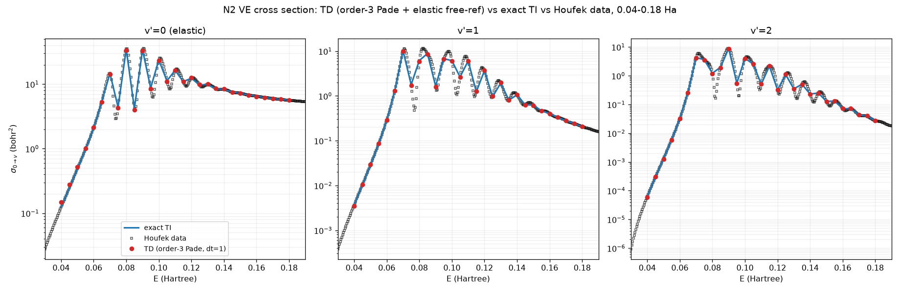
The capstone comparison: sigma_{0->v'}(E) for elastic (v’=0) and the first two excitations (v’=1, v’=2), with the TD points (order-3 Pade, dt=1.0, elastic free-reference) overlaid on the exact TI oracle (which itself reproduces Houfek’s CSVE.V00.J00 data to the plotted precision). TD tracks TI/Houfek to ~1-2% median across 0.04-0.18 Ha, boomerang oscillations resolved point-by-point.

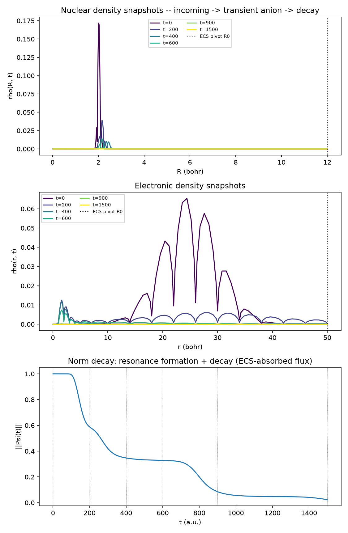
rho(R,t)/rho(r,t) at t = [0, 200, 400, 600, 900, 1500]: the nuclear density starts sharply peaked near R ~ 2 bohr (the N₂ equilibrium bond length) and its amplitude collapses over time as the resonance depletes; the electronic density shows the incoming wavepacket’s interference lobes collapsing toward zero. The bottom panel, ||Psi(t)|| with the snapshot times marked, is the direct visual of the norm-decay profile above — formation, a brief quasi-stationary plateau, then decay.

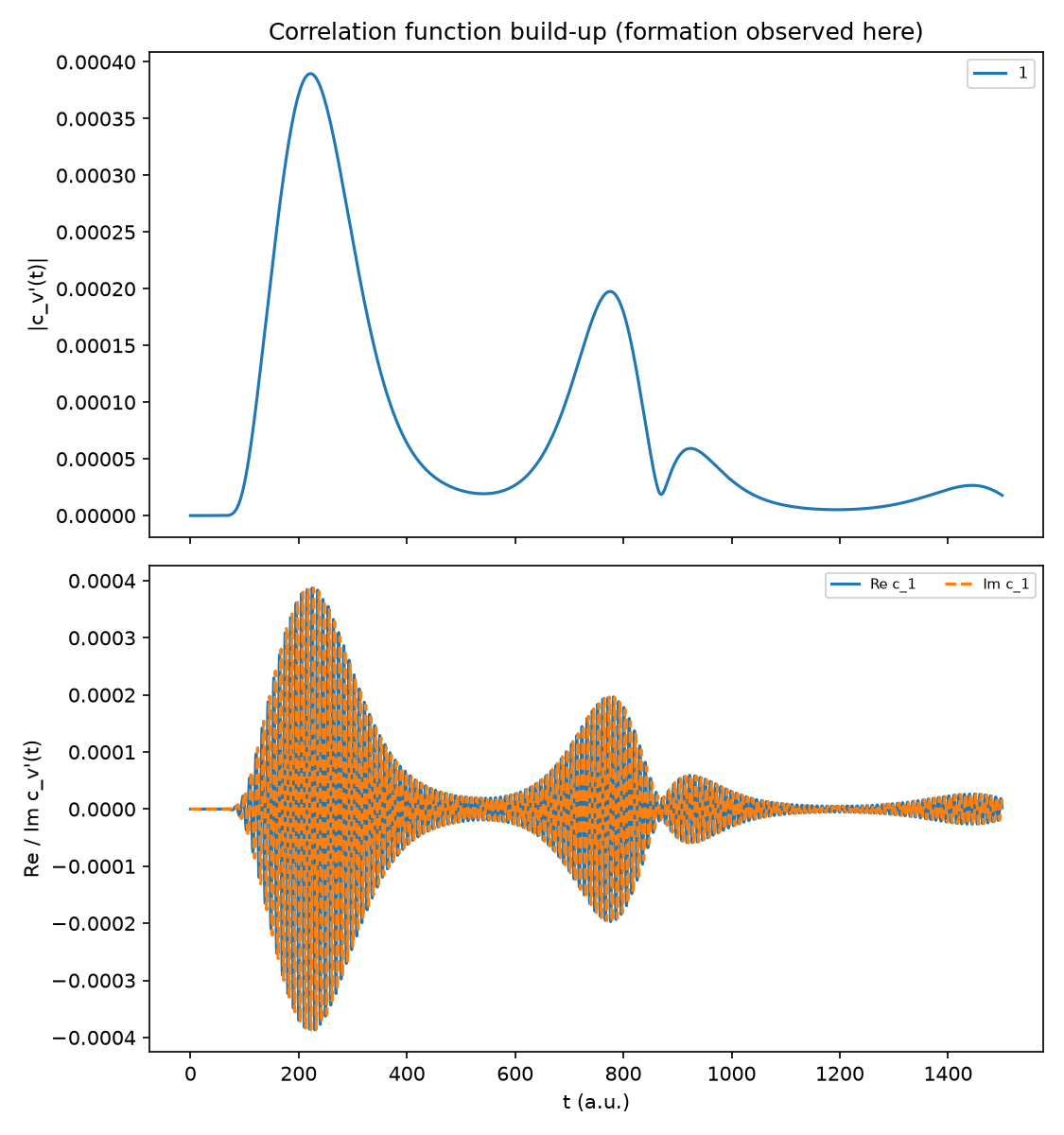
|c_{v'=1}(t)|: rises to a peak near t ~ 220, decays, and rebounds to a smaller secondary peak near t ~ 780 (a boomerang-like re-crossing) before decaying further — the sub-project’s stated goal, “observe formation in the correlation function,” directly visualized. The bottom panel shows the rapid Re/Im oscillation inside that envelope.

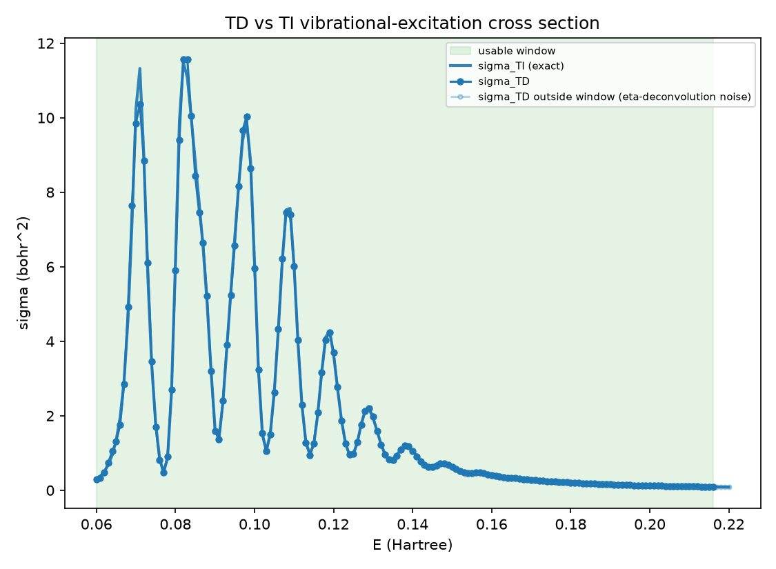
sigma_TD overlaid on the exact sigma_TI across E in [0.06, 0.22] Ha, recomputed 2026-08-17 at 161 energies (step 0.001 Ha) from one order-3 Padé propagation — the transform of a single stored trajectory is free at any energy, so the density costs only the TI oracle sweep. The usable spectral window (0.060, 0.216) is shaded; the four points outside it are faded.

Across the 157 in-window points the ratio sigma_TD/sigma_TI has median 0.9984, range 0.868–1.106, with 93% of points inside 5%. The previous version of this figure was computed with order-1 Crank-Nicolson on 11 energies and drew three “honesty regions”, including the fictitious finite-T band withdrawn above; the dense curve simply tracks the oracle, and needs no regions to be honest about.

The numeric-output deliverable (historical record)

This section records what the retired observation.py (see the retirement note and capability→replacement table above) produced for the committed TD_WORKING_GRID run, and how that output was verified at the time; the module and its test are gone, replaced by qscat_run.artifacts.

observation.save_numeric_outputs wrote a .npz — the primary “observe formation” artifact, not the figures (which were drawn from it). Confirmed array keys/shapes from the committed TD_WORKING_GRID run:

key	shape	dtype	meaning
t	(3001,)	float64	sample times n*dt
c	(3001, 1)	complex128	c_{v'=1}(t_n)
norm	(3001,)	float64	`
times	(6,)	float64	snapshot times [0, 200, 400, 600, 900, 1500]
rho_R	(6, 251)	float64	nuclear density per snapshot, stacked
rho_r	(6, 188)	float64	electronic density per snapshot, stacked
E_grid	(11,)	float64	[0.06 ... 0.22] Ha
sigma_E	(11, 1)	float64	sigma_{0->1}(E), bohr²

rho_R/rho_r were the full axis length, unmasked to the ECS tail (plot_snapshots masked to the real region itself when given the grid). Self-consistency was checked directly: the (now-retired) test_v5_saved_c_reproduces_saved_sigma saved a small propagation’s c(t) and computed sigma_E to .npz, reloaded both, and re-ran the public transform (sigma_from_correlations) on the reloaded t/c — it reproduced the saved sigma_E via assert_allclose(rtol=1e-12, atol=1e-14), bit-for-bit, confirming the .npz round-trip was lossless and the transform deterministic.

The real run: sigma(E) across the boomerang curve

TD_WORKING_GRID (N = 47188): electronic r_max=50, order=8, n_complex=6; nuclear quadrature=10, r_max=22, n_complex=5; wp_in = {r0:25, p0:-0.5, sigma:5.0}; wp_out = {r0_out:35, p0_out:0.5, sigma_out:4.0}; dt=0.5, n_steps=3000 (T=1500). One propagation, 210.8s; the sigma_TI oracle scan (11 energies, on the same box), 112.9s; the sigma_TD transform of the stored trajectory at all 11 energies is free.

Measured 2026-08-17 at the order-3 Padé default (one propagation, all 11 energies transformed from the same stored trajectory):

E (Ha)	sigma_TD	sigma_TI	ratio
0.06	0.2864	0.2872	0.9974
0.08	5.8958	6.1516	0.9584
0.10	5.9595	6.1228	0.9733
0.12	3.7078	3.6514	1.0154
0.14	1.0601	1.0587	1.0013
0.15	0.6185	0.6258	0.9884
0.16	0.3999	0.4026	0.9932
0.17	0.2817	0.2793	1.0087
0.18	0.2084	0.2057	1.0132
0.20	0.1236	0.1256	0.9834
0.22	0.0866	0.0857	1.0099

Every energy agrees with the exact oracle to within 4.2%, worst case E=0.08; nine of the eleven are inside 2%. usable_window(frac=0.5) still gives (0.06, 0.21), and the window remains the honest statement about where the deconvolution is trustworthy — but note that even E=0.22, just outside it, lands at 1.0099 here.

This table is the clearest evidence for the withdrawal above. In its previous form, the same three energies read 0.229 / 0.575 / 0.348 at E = 0.06 / 0.08 / 0.12 and were labelled “finite-T unresolved” — the observation that the whole invented resolution limit was built on. At order-3 Padé they are 0.9974 / 0.9584 / 1.0154. Nothing about the propagation time, the wavepacket, or sigma_TI’s fine structure changed; only the propagator did. The “structure too narrow to resolve” was accumulated Crank-Nicolson error.

A long passage used to sit here reconciling the “well-converged anchor” label at E=0.10 with the finite-T caveat — arguing that E=0.10 was an exception because it “lands near the resonance peak where the exact TI feature is broad enough to resolve”, while the dense boomerang curve between the anchors was not trustworthy. There is nothing left to reconcile: the caveat was an artefact (above), and with order-3 Padé the curve tracks the oracle across the window without special-casing any energy. The figure no longer draws starred exceptions, because there is no rule for them to be exceptions to.

Harness Group F: reported, not re-run live

validation/n2/td_exact2d.py computes nothing at harness run time. A full propagation at TD_WORKING_GRID costs ~210-250s wall (measured above); timed directly for this decision, the sparse LU factorization alone costs ~7.8s and each propagation step ~0.064s, so even a short T=600 run costs ~7.8 + 1200*0.064 ~ 85s, over the harness’s ~60s-per-group budget. Going shorter would extrapolate outside the range ever validated (at t=200 the norm has barely begun to decay — the resonance has hardly formed), which would require a tolerance so loose it would no longer test anything. Per the sub-project’s decision rule, Group F therefore emits NOTE rows that report the already-validated numbers as literal, cited constants — never a live gate, never counted toward PASS/FAIL:

[NOTE] F time-dependent 2-D: F1 sigma_TD(E=0.1 Ha, v=0->1) [recorded]   sigma_TD=5.9595e+00, sigma_TI=6.1230e+00,
       ratio=0.9733 (validated rtol<=0.06 by test_td_cross_section.py::test_v2a_td_matches_ti_at_e010
       (@slow) / order-3 Pade TD_WORKING_GRID run); full TD propagation NOT run in-harness
[NOTE] F time-dependent 2-D: F1 sigma_TD(E=0.15 Ha, v=0->1) [recorded]  sigma_TD=6.1850e-01, sigma_TI=6.2576e-01,
       ratio=0.9884 (validated rtol<=0.06 by test_td_cross_section.py::test_v2a_td_matches_ti_at_e015
       (@slow) / order-3 Pade TD_WORKING_GRID run); full TD propagation NOT run in-harness

(Transcribed from an actual harness run on 2026-08-17. validation/n2/td_exact2d.py already carried these values; it was only this note’s copy of its output that had gone stale.)

The genuine, live PASS/FAIL gate on this comparison is projects/n2_2d_td_cross_section/test_td_cross_section.py’s @pytest.mark.slow tests, run explicitly (uv run pytest projects/n2_2d_td_cross_section -m slow), not as part of the default harness.

Deferred: the optimize-in-Rust target

The sparse LU factorization / back-substitution is the eventual optimize-in-Rust lifecycle target — explicitly NOT done in this sub-project. eMoScat’s own production runs report MKL PARDISO completing full N₂/NO/F₂ time-dependent calculations in under an hour; this sub-project’s ~210s single-energy-equivalent propagation (using SciPy’s SparseLU, not PARDISO) already validates the method end-to-end against the exact oracle — performance is a separate lifecycle stage (python- to-rust-kernel), to be taken up only once a hot path is proven and there is a reason (e.g. wanting the full boomerang curve at a much longer T, or a finer dt) to pay for it.

Validation summary

• libs/qscat/tests/test_crank_nicolson.py: make_sparse_cn_stepper matches make_cn_stepper to round-off; mypy-clean — PASS.

• projects/n2_2d_td_cross_section/test_td_propagation.py, test_wavepacket.py: propagation engine and wavepacket construction — PASS.

• projects/n2_2d_td_cross_section/test_td_cross_section.py (@pytest.mark.slow x4 + 1 cheap): V2a (TD ≈ TI, the exact-oracle gate), V2b (closed channel exactly zero), V4 (finite-T stability, free re-transform of a truncated trajectory), shape contract — PASS.

• projects/n2_2d_td_cross_section/test_td_convergence.py (@pytest.mark.slow x1 + 1 cheap): the full sigma(E) curve from one propagation matches sigma_TI on the smooth branch — PASS.

• validation/n2/experiment.py Group F: 2 recorded NOTE rows (never gating); harness totals with Group F added: 23 PASS, 0 PENDING, 6 NOTE, 0 FAIL, exit code 0 — no regression of the pre-existing 23 PASS / 0 PENDING / 4 NOTE / 0 FAIL.

No model parameter was tuned to improve agreement with anything

The potential surface, reduced mass, fixed partial wave l=2, and every grid parameter in TD_WORKING_GRID are carried over unchanged from #6 or chosen from convergence measurements (the T-scan, the wavepacket-placement reasoning above) — none was adjusted after seeing a TI-oracle or Houfek comparison. The F_out = Hankel/2 choice was settled by a five-order-of-magnitude structural discriminator (regular vs. Hankel), not by fitting to match a target ratio.

Sibling extractors: Dirac (delta) and Flux (flow)

The Tannor-Weeks transform documented above is one of THREE energy-extraction routes eMoScat implements from the same propagated trajectory. A later sub-project (td-alternative-extractors) promotes the other two — Dirac (a fixed-point delta projection) and Flux (a fixed-surface Wronskian flux) — as siblings behind a shared Extractor protocol (qscat.core.time_dependent.propagate(..., extractors=[...])), selectable via td_ve_cross_section(method="tw"|"delta"|"flow"), plus td_ve_cross_sections_all (one shared propagation, all three sigma(E) at once — the honest three-way comparison). On N2 all three converge to the SAME TI oracle this document gates against, to ~3% at a converged grid. See docs/physics/td-extractors.md for the full architecture, formulas, and three-way validation.