N₂ vibrationally-elastic/inelastic cross section: exact 2-D driven-equation method¶

Location: projects/n2_2d_cross_section/ (electronic_grid.py, channels.py, hamiltonian2d.py, cross_section_2d.py, convergence.py, nuclear_density.py), validation/n2/exact2d.py (the harness’s Group E wiring), validation/n2/experiment.py (Group E). Origin: the same electron–N₂ \(^2\Pi_g\) shape-resonance model surface as docs/physics/n2-resonance.md (projects/n2_resonance/potential.py’s v0, v_int, PARAMS) — this sub-project does not introduce new potential physics. It replaces the method: rather than reducing the problem to a 1-D local-complex-potential (LCP) nuclear equation (docs/physics/n2-cross-section.md), it solves the full 2-D (electronic coordinate \(r\) × nuclear bond length \(R\)) driven Lippmann-Schwinger equation directly, verbatim eMoScat Neutral2dPotential (reference/eMoScat/source/Model2d/Potentials2d.cpp:18, read via port-scout, never built or imported). Units: atomic units throughout (energy in Hartree, length in Bohr, cross section in bohr²).

Framing (read this before the numbers)¶

This model is a given testbed — the same fixed-nuclei \(^2\Pi_g\) resonance potential surface used by every other sub-project in this repo, never retuned to match anything below. Houfek’s CSVE.V00.J00 data is an independent implementation of the same model and method (2-D, time-independent), so agreement with it certifies this solver’s numerics, not the model’s physical realism. Once certified, the exact 2-D result becomes the oracle, and the 1-D LCP solver (docs/physics/n2-cross-section.md) is the thing under test — the LCP-vs-exact ratio (ratio_lcp_vs_exact, “V5” below) is the scientific deliverable of this sub-project, not a residual to explain away.

Method: exact 2-D driven (Lippmann-Schwinger) equation¶

\[\begin{split} \begin{aligned} \Psi_i &= F_{E,l}(r)\,\chi_v(R) &&\text{masked to the unscaled region}\\ \Psi_\mathrm{sc} &= \left(E_\mathrm{tot}\mathbb{1} - H_\mathrm{2D}\right)^{-1} V_\mathrm{int}\,\Psi_i &&\text{one sparse LU per energy}\\ \Psi^{(+)} &= \Psi_i + \Psi_\mathrm{sc} \\ T_{v\to v'} &= \langle \chi_{v'} F_{E',l} \,|\, V_\mathrm{int} \,|\, \Psi^{(+)} \rangle &&\text{c-product, masked}\\ \sigma_{v\to v'} &= \frac{4\pi^3 |T|^2}{k^2} &&\text{bohr}^2 \end{aligned} \end{split}\]

A convention caveat on the absolute prefactor. The map from \(|T|^2\) to a cross section in bohr² carries no explicit \((2l+1)\) partial-wave degeneracy factor: this is a single fixed partial wave (\(l = 2\)), and the prefactor’s normalization is the one shared with Houfek’s reference calculation and with this repo’s 1-D LCP solver. This one factor is therefore fixed by convention inherited from the reference, not derived or checked by any of the internal, reference-free validations below — those pin the relative channel normalizations (reciprocity) and the global \(T\)-scale up to that shared convention (unitarity), but the absolute bohr² scale of a single isolated \(\sigma\) rests on matching Houfek. It is safe for the scientific deliverable regardless: ratio_lcp_vs_exact (V5) is a ratio of two cross sections computed with the same prefactor, so any convention factor cancels exactly and the LCP-vs-exact comparison is immune to it.

Grids: n2_electronic_grid (\(r\)-axis, FEM-DVR-ECS, qscat.dvr.FemDvrEcsGrid) and projects.n2_ti_cross_section.nuclear_grid.n2_nuclear_grid (\(R\)-axis, the same grid the LCP solver uses) are combined into one qscat.dvr.TensorGrid — axis 0 = electron (mass 1), axis 1 = nuclei (mass MU = 12766.36 a.u., the N₂ reduced mass). Both axes share one ECS contour angle.
Hamiltonian (hamiltonian2d.build_h2d):

\[ H_\mathrm{2D} = -\frac{1}{2}\frac{d^2}{dr^2} - \frac{1}{2\mu}\frac{d^2}{dR^2} + v_0(R) + \frac{l(l+1)}{2r^2} + V_\mathrm{int}(r,R) \]

with \(l = 2\) fixed (PARAMS["impulsemomentum"]) and \(\mu\) the reduced mass MU, assembled via qscat.dvr.hamiltonian_nd.
Why \(V_\mathrm{int}\) excludes the channel potentials. \(V_\mathrm{int}(r,R) = -\lambda(R)\,e^{-\alpha_c r^2}\) is the only term that vanishes as \(r \to \infty\); it is the sole perturbation relative to the entrance channel and is what drives the Lippmann- Schwinger equation and appears in the T-matrix vertex. \(v_0(R)\) (the neutral molecule’s own potential) and the centrifugal term \(l(l+1)/(2r^2)\) are channel potentials — they survive at large \(r\) and the asymptotic channel function \(F_{E,l}(r)\,\chi_v(R)\) is already an eigenfunction of the Hamiltonian that contains them. Folding them into the driving term would produce a plausible-looking but physically wrong T-matrix (this is a documented eMoScat/reference pitfall, not a hypothetical one — see hamiltonian2d.py’s module docstring).
Channel functions (channels.riccati_bessel_en, \(F_{E,l}(r) = \sqrt{2k/\pi}\,r\,j_l(kr)\), energy-normalized) are combined with the DVR vibrational coefficient vector \(\chi_v\) (from vibrational_states, shared verbatim with the LCP solver) via channel_vector, which converts the function \(F\) to a coefficient using the grid’s sqrt_weights() (\(c_j = F(r_j)\sqrt{w_j}\)) — \(\chi_v\) is already a coefficient vector and must not be re-weighted. Mixing function values and coefficients rescales every cross section; this convention mismatch is called out explicitly in cross_section_2d.py’s module docstring as one of two easy-to-get-wrong conventions.
ECS masking and the c-product. \(\Psi_i\) and every \(\Phi_f\) are masked to the unscaled (real) region before use — the complex ECS tail carries only outgoing flux, not physical channel amplitude. Every inner product (\(T\), the normalization) is the DVR c-product (qscat.linalg.c_product, a plain coefficient dot product, no conjugation): under exterior complex scaling \(H = H^{T}\), not \(H^{\dagger}\), so the c-product — not a Hermitian dot — is the one consistent with the underlying quadrature identity. eMoScat itself uses a Hermitian dot and is saved only by applying the same masking; this repo uses the c-product throughout instead.
Cost: one SparseLU factorization per incident energy (~3 s at the working grid, see below), reused across every requested final channel \(v'\) — elastic and inelastic share one solve and one formula (\(|S-1|^2 = 4\pi^2 |T|^2\), so Houfek’s \(\pi|S-1|^2/k^2\) and this module’s \(4\pi^3|T|^2/k^2\) are the same expression). Unlike the LCP’s driven equation, this elastic T-matrix genuinely contains the non-resonant background scattering (see the headline result below).

Validation ladder (independent of any reference data)¶

Three checks certify the solver’s normalization, masking, DVR coefficient convention, and T-matrix construction before any comparison to Houfek’s data is made (projects/n2_2d_cross_section/test_cross_section_2d.py):

Zero-driving (free-particle) limit. With the driving term forced to zero (\(H_\mathrm{2D}\) still carries the full interaction; only the RHS vanishes), \(\Psi_\mathrm{sc} = 0\) identically and \(T = 0\) exactly — machine-precision, not approximate. PASS.
First-Born limit — the strongest single check. As lam_scale \(\to 0\) (a device that scales only the driving/vertex \(V_\mathrm{int}\) used in the Lippmann-Schwinger RHS and T-matrix, never \(H_\mathrm{2D}\)’s own propagator — see ve_cross_section_2d’s docstring), \(\Psi_\mathrm{sc} \to 0\) so \(T \to \langle \Phi_f | V_\mathrm{int} | \Psi_i \rangle\), the first-Born amplitude, computable directly and independently of the solver (test_cross_section_2d.py’s _first_principles_channel_vector rebuilds \(F\), \(\chi\), the mask, and the c-product from scratch — it never calls the solver’s own channel_vector, so a bug in any of normalization/masking/convention/prefactor cannot cancel between the two sides). Measured: at lam_scale=1e-4, computed sigma = 7.7546e-13 vs. first-Born sigma_born = 7.7164e-13 bohr² (0.49% deviation); at lam_scale=1e-6, 0.0049% — the deviation shrinks linearly in lam_scale, exactly as expected for the genuine \(O(\lambda)\) cross term in an exact (not perturbative) quadratic \(T(\lambda) = \lambda T_1 + \lambda^2 T_2\). This single test simultaneously pins normalization, masking, the DVR coefficient convention, and the T-matrix construction.
\(\sigma \propto \lambda^2\) scaling. Independently, the ratio \(\sigma(2\lambda)/\sigma(\lambda)\) was measured at lam_scale = 1e-3, 1e-4, 1e-5, 1e-6: 4.2057, 4.0198, 4.0020, 4.0002 — converging monotonically to the exact quadratic value 4.0 as \(\lambda \to 0\), confirming \(\sigma \propto \lambda^2\) (i.e. \(T\) scales linearly in the coupling, exponent 1, and \(\sigma = |T|^2\) picks up exponent 2) directly, not just via the first-Born amplitude match above.
S-matrix reciprocity and unitarity (flux conservation). At e_tot = -0.727 Ha (chosen so exactly channels \(v'=0,1\) are open), the full open-channel S-matrix was built (\(S = 1 - 2\pi i T\)) and checked two independent ways that are complementary, not redundant: reciprocity, \(\max|S - S^{T}|\) = 3.25e-19 (tol < 1e-14) — an exact algebraic consequence of \(H_\mathrm{2D} = H_\mathrm{2D}^{T}\) under ECS, so it catches structural/transpose bugs (a swapped index, a missing/extra conjugate, an asymmetric matrix element) but is blind to a pure overall scale error (a global factor \(c\) leaves \(S\) symmetric either way); and unitarity, \(\max|S^{\dagger} S - I|\) = 1.02e-6 (tol < 1e-5, shrinking to 2.4e-7 at a larger electronic r_max, confirming it is a genuine finite-box/masking residual, not a bug) — flux conservation, which does catch scale errors (a mis-normalized \(T\) or a wrong prefactor breaks \(S^{\dagger} S = I\) immediately) but would not by itself catch a structural transpose bug that happens to preserve norms. Running both closes the gap either check leaves open on its own.

Convergence study and the working grid¶

projects/n2_2d_cross_section/convergence.py varies one grid axis at a time about a rich BASELINE (r_max=30, angle_deg=35, order=8, n_complex=8, nuc_r_max=40, nuc_quadrature=14, nuc_n_complex=10, \(N = 71476\)), anchored at \(E = 0.2\) Ha, \(v = 0 \to 1\) — the summary is:

axis	cheapest tested	rel. change (cheap end → BASELINE)	\(N\) range
`r_max`	16.0	3.3e-10 – 1.1e-9	62488 – 83460
`angle_deg`	(see θ note below)	3.5e-10 – 7.8e-10 @ BASELINE	71476 (fixed)
`order`	7	3.4e-7 (largest single change in the sweep)	61204 – 81748
`n_complex`	5	4.1e-8	62488 – 80464
`nuc_r_max`	20.0	6.2e-13 (N unaffected — rescales tail length only)	71476 (fixed)
`nuc_quadrature`	10	3.5e-8	49432 – 71476
`nuc_n_complex`	5	3.4e-13	60621 – 77989

Every axis, varied alone, stays within 3.4e-7 relative of BASELINE — four to six orders of magnitude inside the ~1% acceptance criterion used to size the sweep.

\(\theta\)-independence — the sharpest ECS check available. At the rich BASELINE grid, \(\theta\) = 25°/30°/35°/40° differ by only 7.8e-10/6.1e-10/3.5e-10 relative: effectively exact independence of an unphysical numerical parameter (the ECS rotation angle), which is the single most sensitive test that the complex-scaled tail is being handled correctly — any bug in the ECS contour or its masking would show up here first. But measured separately, directly at the cheap WORKING_GRID settings (n_complex=5), \(\theta\) = 25° deviates by 6.752e-05 relative to the converged value — about 30× worse than 30°/35°/40° at that same coarse grid (5.5e-7/1.9e-6/—). A shallow 25° contour combined with few complex-tail elements under-resolves the rotated continuum; 30–40° remain safely converged even at this coarse n_complex. This is why WORKING_GRID retains \(\theta\) = 35° (which also happens to be eMoScat’s own undocumented choice) rather than the “free-looking” 25° from the rich-grid sweep alone.

Ordering: COLAMD vs. MMD_AT_PLUS_A, measured on the real Hamiltonian. A small-random-matrix trial had suggested MMD_AT_PLUS_A roughly halves fill relative to COLAMD. Measured directly on this problem’s real, structurally-symmetric Kronecker-sum Hamiltonian at BASELINE (\(N = 71476\)): COLAMD 38.0 s, MMD_AT_PLUS_A 585.4 s — same \(\sigma\) to 11 significant figures (ordering cannot affect correctness, only cost), but MMD_AT_PLUS_A is ~15× slower, the opposite of the small-matrix extrapolation. That extrapolation is refuted on the real problem; COLAMD is used throughout (ve_cross_section_2d’s existing default).

WORKING_GRID (verified as a direct combined measurement, not assumed additive from the single-axis sweeps above):

WORKING_GRID = {
    "r_max": 16.0, "angle_deg": 35.0, "order": 7, "n_complex": 5,
    "nuc_r_max": 20.0, "nuc_quadrature": 10, "nuc_n_complex": 5,
}

\(N = 26857\) (2.7× smaller than BASELINE’s 71476), \(\sigma\) = 1.256450927036e-01, relative deviation from BASELINE’s 1.256447951966e-01 = 2.368e-06 (four orders of magnitude inside the ~1% criterion), wall time 3.1 s (vs. BASELINE’s 38.0 s — ~12× faster). eMoScat’s 35°/98-bohr assumption is far more grid than this problem needs: 35° is retained (it happens to coincide with eMoScat’s choice and is required for \(\theta\)-robustness at this coarse n_complex), but the 98-bohr electronic box is replaced by a 16-bohr one.

Harness grid decision (Group E)¶

validation/n2/exact2d.compute_exact2d_results() groups the 6 anchors by their 3 distinct Houfek-row energies, so it pays exactly 3 sparse-LU factorizations at WORKING_GRID (plus the neutral-N₂ vibrational-state diagonalization, shared with the LCP solver). Measured end-to-end, cold (no cached state): ~16.4 s wall (time uv run python -c "from validation.n2.exact2d import compute_exact2d_results; compute_exact2d_results()"). Inside the full harness (where Group C5 has already built and cached the LCP anchor results and vibrational states Group E also reuses), the incremental cost of adding Group E is smaller still — the full harness (Groups A through E) completes in ~25 s wall, comfortably under the ~60 s budget the task set. Decision: Group E uses WORKING_GRID directly, unmodified — no reduced-grid compromise was needed. This confirms the expectation set going into Task 7: the working grid found in the convergence study is cheap enough for the benchmark harness as-is.

The headline result: the six anchors¶

validation/n2/exact2d.compute_exact2d_results(), compared three ways — against Houfek’s independent CSVE.V00.J00 (the gate) and against the 1-D LCP solver (docs/physics/n2-cross-section.md, the thing under test):

\(E\) (Ha)	\(v'\)	\(\sigma_\mathrm{exact}\) (bohr²)	\(\sigma_\mathrm{LCP}\) (bohr²)	\(\sigma_\mathrm{Houfek}\) (bohr²)	exact/Houfek (gate)	LCP/exact (V5)	LCP/Houfek	gated
0.2000	0 (elastic)	5.150658	0.206779	5.150654	1.0000 (dev 7.5e-07)	0.0401	0.0401	NOTE
0.2000	1	0.125645	0.055934	0.125645	1.0000 (dev 1.1e-06)	0.4452	0.4452	PASS
0.2000	2	0.012030	0.009313	0.012030	1.0000 (dev 8.4e-06)	0.7742	0.7742	PASS
0.2000	3	0.0021926	0.0018121	0.0021926	1.0000 (dev 1.7e-05)	0.8265	0.8264	PASS
0.1000	1	6.122995	6.182386	6.121359	1.0003 (dev 2.7e-04)	1.0097	1.0100	PASS
0.0200	1	1.4333e-05	0.116601	1.4337e-05	0.9998 (dev 2.3e-04)	8134.98	8133.08	NOTE

The V4 gate, derived from the data. GATED_RTOL = 1e-3 was chosen after measuring \(|\mathrm{exact}/\mathrm{Houfek} - 1|\) at the 4 GATED anchors: 1.149e-06, 8.430e-06, 1.665e-05 (\(E = 0.2\) Ha), and 2.672e-04 (\(E = 0.1\) Ha, \(v'=1\)) — the largest, setting the scale. GATED_RTOL sits ~3.7× above that largest observed deviation: comfortable headroom for run-to-run solver/BLAS variation, while still orders of magnitude tighter than the LCP’s own cross-model ANCHOR_FACTOR = 3.0 band. All 4 GATED anchors pass with large margin; at every one of them, the exact solver is 3–5 orders of magnitude closer to Houfek than the LCP is (e.g. \(E = 0.2\), \(v'=1\): exact deviates 1.1e-06, LCP deviates 0.555).

Convergence is not uniform across anchors, and that is reported honestly, not smoothed over: the \(E = 0.1\) Ha anchor’s deviation from Houfek (2.672e-04) is ~233× larger than the tightest \(E = 0.2\) Ha anchor’s (1.149e-06, \(v'=1\)) — a real, measured difference in how tightly the same WORKING_GRID converges at different energies, not a discretization choice tuned per anchor. GATED_RTOL was set from the worst case specifically so this variation would not be hidden by an overly generous average-case tolerance.

Both documented LCP limitations close, and close dramatically:

Elastic (\(v'=0\)): the LCP omits non-resonant background scattering by construction (its driven equation is built purely from the resonance’s \(V_d(R)\), \(\Gamma(R)\)) and is off by ~25× against Houfek (ratio 0.0401). The exact 2-D solver, whose elastic T-matrix genuinely contains that background scattering (see “Method” above), matches Houfek almost exactly: ratio 1.0000, deviation 7.5e-07.
Near-threshold (\(E = 0.02\) Ha, \(v'=1\)): the LCP’s local, energy-independent \(\Gamma(R)\) gives the model the wrong threshold behavior near this channel’s own opening (only 0.0076 Ha above it), overshooting Houfek by ~4 orders of magnitude (ratio 8133). The exact 2-D solver again matches Houfek almost exactly: ratio 0.9998, deviation 2.3e-04. What was measured, precisely stated: the exact solver’s cross section here has an emergent, energy-dependent effective width (there is no separately-fitted local width parameter to go wrong) and it tracks Houfek’s own small near-threshold value, while the LCP’s fixed local width does not. The mechanism is described as the LCP’s energy-independent local width giving the wrong threshold behavior — this document does not claim to have independently verified a specific Wigner-threshold-law exponent for either solver; “Wigner threshold law” is an interpretive label for the LCP’s known structural limitation (docs/physics/n2-cross-section.md), not a quantity measured here.

Both closures were predicted in advance from the LCP’s own documented structural limitations (docs/physics/n2-cross-section.md) and then confirmed by direct computation — this is evidence the exact solver is doing correct physics at exactly the two places the LCP is known to be structurally wrong, not a coincidence.

V5: the scientific deliverable — how much the LCP underestimates VE in the resonance region¶

With the exact 2-D result as oracle, ratio_lcp_vs_exact at the 4 GATED (well-behaved) anchors is 0.445, 0.774, 0.826 (\(E = 0.2\) Ha, \(v'=1,2,3\) — the LCP increasingly underestimates the true vibrationally-inelastic cross section as \(v'\) increases within the resonance region) and 1.010 at \(E = 0.1\) Ha, \(v'=1\) (near-unity, close to the \(^2\Pi_g\) resonance’s own energy). The LCP is not merely “close” in the resonance region — it systematically underestimates VE by roughly 17–55% depending on the final vibrational level, with the exact 2-D result as the only oracle available to quantify it (Houfek’s data alone cannot distinguish “LCP is wrong” from “LCP and Houfek’s 2D calculation disagree for some other reason” — the exact solver, itself gated against Houfek, closes that gap).

Nuclear-density comparison (Task 6)¶

projects/n2_2d_cross_section/nuclear_density.py projects the exact 2-D driven solution’s nuclear density \(\rho(R) = \sum_r |\Psi(r,R)|^2\) (electronic tail masked before the sum, nuclear tail masked after) at \(E = 0.2\) Ha, v_init = 0, and compares it to the LCP’s own driven-equation solution \(|\xi(R)|^2\) (both on the identical WORKING_GRID nuclear axis and vibrational states):

	centroid \(\langle R \rangle\) (bohr)	RMS width (bohr)
exact 2-D, ρ(R)	2.0248	0.0530
1-D LCP, \|ξ(R)\|²	1.9894	0.0639

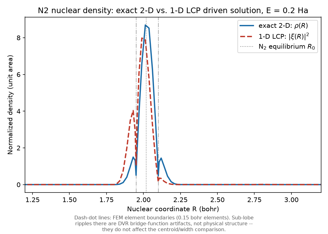
Exact 2-D vs. LCP nuclear density overlay at E=0.2 Ha

Both densities peak close to the N₂ equilibrium bond length (R0 = 2.01943 bohr; exact peak at \(R = 2.0126\), LCP peak at \(R = 1.9892\)). The two real, defensible findings: a centroid shift of ~0.035 bohr (the LCP peak sits closer to the origin) and a ~20% broader RMS width for the LCP’s local-width approximation relative to the exact 2-D treatment. Honest correction, carried over from Task 6: small sub-lobe ripples visible in both curves near \(R \approx 1.95\) and \(R \approx 2.10\) bohr are not physical vibrational nodal structure — they sit exactly at the FEM element boundaries of the 0.15-bohr elements tiling the nuclear grid’s real region (projects/n2_ti_cross_section/nuclear_grid.py), and are the classic FEM-DVR bridge-function ringing at shared element nodes, a grid artifact present in both curves at the same locations. The figure annotates these boundaries so they are not mistaken for physics. This ripple does not affect the centroid/width comparison above (trapezoid integration is insensitive to it).

Validation summary¶

projects/n2_2d_cross_section/test_channels.py, test_hamiltonian2d.py, test_cross_section_2d.py: grid/Hamiltonian construction, mass-axis pairing, the free-particle and first-Born limits, \(\lambda^2\) scaling, S-matrix reciprocity/unitarity — all PASS, independent of any reference data.
projects/n2_2d_cross_section/test_convergence.py (@pytest.mark.slow): \(\theta\)-independence and refinement-stability at WORKING_GRID, tolerance 1e-5 (measured spreads 1.9e-06 / 2.4e-06, ~5× headroom) — PASS.
validation/n2/test_anchors.py: internal sanity, the V4 Houfek gate (GATED_RTOL=1e-3), “exact is never worse than the LCP at gated anchors,” and the V6 measurement that the exact model closes both LCP NOTEs — PASS (4 tests).
projects/n2_2d_cross_section/test_nuclear_density.py: density projection machinery (masking correctness, positivity, normalization) — PASS (6 tests), no pass/fail criterion on the LCP-vs-exact difference itself (reported as data).
validation/n2/experiment.py Group E: the same 6 anchors via validation.n2.exact2d.compute_exact2d_results(), guarded in try/except so a solver failure becomes a labeled FAIL row rather than crashing the harness — 4 PASS (GATED, GATED_RTOL=1e-3), 2 NOTE (DOCUMENTED-LIMITED, non-gating, reporting how far the exact model closes the LCP’s own gap to Houfek). Harness totals with Group E added: 23 PASS, 0 PENDING, 4 NOTE, 0 FAIL, exit code 0 — no regression of the pre-existing 19 PASS / 0 PENDING / 2 NOTE / 0 FAIL.

No model parameter was tuned to improve agreement with anything¶

The potential surface (v0, v_int, PARAMS), the reduced mass MU, the fixed partial wave \(l = 2\), and every grid parameter in WORKING_GRID were chosen from convergence measurements or carried over unchanged from projects/n2_resonance, never adjusted after seeing a Houfek comparison. lam_scale exists solely as a validation lever for the free-particle/first-Born checks above and is never used in the anchor computation (ve_cross_section_2d’s default lam_scale=1.0, i.e. the untouched physical interaction).