The time-dependent nonlocal resonance model

The time-domain sibling of docs/physics/nonlocal-resonance-model.md. Same model, same ingredients, same grids — a second, independent route to the same \(\Psi_d\), and a set of observables the first route cannot produce.

Method: Gertitschke & Domcke, Phys. Rev. A 47, 1031 (1993) (reference/literature/gertitschke-1993-pra47-1031.md), applied to the model of Houfek, Rescigno & McCurdy, Phys. Rev. A 77, 012710 (2008) (reference/literature/houfek-2008-pra77-012710.md). Propagator: the order-3 diagonal Padé of van Dijk & Toyama, Phys. Rev. E 75, 036707 (2007), already shipped as qscat.evolution.make_pade_stepper.

1. Why, given that it is slower

It is slower — measurably. One F₂ propagation costs ~0.3–0.8 s per step over ~6000 steps; the resolvent answers the same energies in a fraction of that. The time-dependent route is not justified on cost and this note does not claim it is.

It is justified because a resolvent returns \(\Psi_d(R;E)\) and says nothing about how the collision complex reached it. A propagation returns \(\Psi_d(R,t)\), and with it the survival, the centroid and the mean momentum — the quantities that turn a cross-section feature into a mechanism. Váňa & Houfek, Phys. Rev. A 95, 022714 (2017) is built on exactly that: the correspondence between individual peaks and quasibound states, the several time-separated contributions behind an asymmetric peak, and the formation-time argument for NO’s long-lived structure (pp. 022714-13, -15). Gertitschke & Domcke’s own headline result is of the same kind — their explanation of why the LCP fails for H₂⁻ is a temporary packet splitting between ≈2 and ≈5 fs, invisible in any energy-domain calculation (p. 1041).

PRA 95 proposes this work in its closing paragraph: similar time-dependent calculations “could be performed within the LCP approximation or the nonlocal resonance model and thus interpret the results in the same way”, offered as a future direction and not executed there (p. 022714-16).

2. The formulation

2.1 The memory integral, and why it is not solved as one

PRA 47 Eq. (2.1) is non-Markovian:

i ∂_t Ψ_d(R,t) = [T_N + V_d(R)] Ψ_d(R,t)
                 + (1/i) ∫_0^t dt' ∫ dR' F(R,R',t−t') Ψ_d(R',t')

Evaluated literally this is O(N_t²) and needs the kernel at every lag. It does not have to be. The kernel this repository builds (nrm.nonlocal_potential.nonlocal_operator, PRA 77 Eq. 60–61) is already a sum of resolvents:

F(E) = Σ_n diag(V_dn) · (E − H_n)^{-1} · diag(V_dn)
H_n  = T_R + V_0(R) + E_n(R)

2.2 The resummation

Introduce one auxiliary nuclear packet \(\phi_n\) per projected electronic state. The pair \((\Psi_d, \{\phi_n\})\) obeys a time-local system:

i ∂_t Ψ_d = (T_N + V_d) Ψ_d + Σ_n V_dn φ_n
i ∂_t φ_n = H_n φ_n + V_dn Ψ_d

i.e. propagation under one block Hamiltonian on (1 + n)·N_R unknowns:

        ⎡ T_N + diag(V_d)   diag(V_d1)           diag(V_d2)          … ⎤
H_ext = ⎢ diag(V_d1)        T_N + diag(V_0+E_1)   0                  … ⎥
        ⎣ diag(V_d2)        0                     T_N + diag(V_0+E_2)  ⎦

sparse (every off-diagonal block is diagonal), complex symmetric (ECS, never Hermitian), and energy-independent.

This is Eq. (2.1) resummed, not approximated. Eliminating the auxiliary blocks from the time-independent version, \(\phi_n = (E - H_n)^{-1} V_{dn} \Psi_d\), returns PRA 77 Eq. (52) with exactly the F(E) above. Verified numerically: the d-block of (E − H_ext)^{-1} matches (E − T_N − V_d − F(E))^{-1} to 4.4e-14 relative (F₂, N_R = 584, cond ≈ 1.1e6).

2.3 Back to the frequency domain

For \(i\,\partial_t\Psi = H_\mathrm{ext}\Psi\) with \(\Psi(0)\) given, integrating ∫_0^∞ dt e^{i(E+i0)t} by parts and killing the t→∞ boundary term by ECS absorption,

(E − H_ext) Ψ̂(E) = i Ψ(0)      ⟹      Ψ̂(E) = i (E − H_ext)^{-1} Ψ(0)

With \(\Psi(0) = (\xi, 0, 0, \ldots)\) and \(\xi = V_{dk_i}(R)\,\chi_{v_i}(R)\) — PRA 47 Eq. (2.5), and byte-identical to the right-hand side the time-independent route already builds for Eq. (52) — the d-block gives

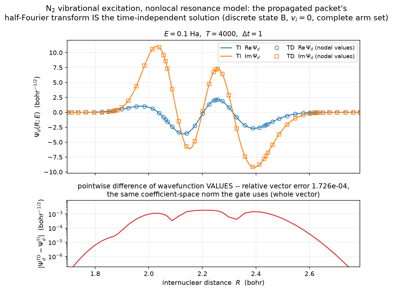
Ψ_d^TI(R;E) = −i ∫_0^∞ dt e^{iEt} Ψ_d(R,t)

The −i is derived here and confirmed independently by PRA 47 Eq. (2.6), whose (1/i) makes \(T_{v'v}(E) = \langle \chi_{v'} V_{dk_f} | \Psi_d^\mathrm{TI} \rangle\) — precisely the shipped vibrational_excitation.t_resonant.

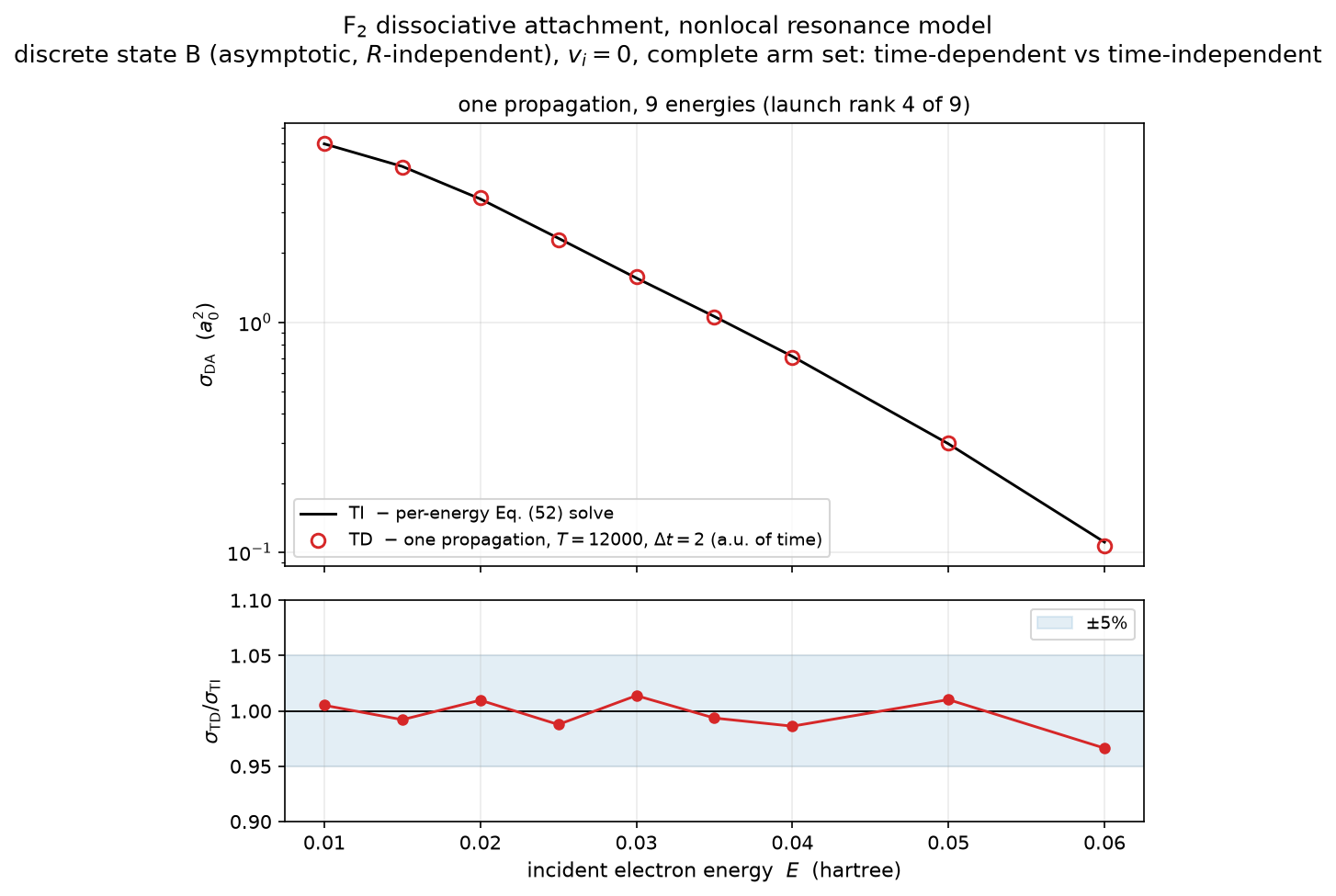
The consequence is the design. The time-dependent route produces the same nuclear vector the time-independent route produces, so every downstream step is existing, tested code: dissociation.da_sigma_from_psi for DA, t_resonant + t_background for VE. No cross-section normalization is re-derived, and the conjugation conventions settled for the TI route (PRA 77 Eq. 34/35 collapsing V^{−*}_{dk} to a non-conjugated V^+_{dk}; Eq. 37’s bra carrying \(\phi^+\) at the final channel energy) are inherited rather than re-litigated.

2.4 One propagation for every energy

\(\xi\) depends on the incident energy through V_dk_i, so exact algebra says one launch state per energy. PRA 47 Eq. (2.17) removes that by rescaling with \([\Gamma(E_i)/2\pi]^{-1/2}\), under the separability \(\Gamma(E,R) = \Gamma(E)\,g(R)^2\) of Eq. (2.16) — which the Houfek models do not satisfy exactly.

They satisfy it numerically. Because \(\alpha_c\) is a constant in \(V_\mathrm{int}(r,R) = -\lambda(R)e^{-\alpha_c r^2}\), the whole R-dependence of the electronic problem enters through the single scalar \(\lambda(R)\) — \(H_\mathrm{el}(R) = H_0 + \lambda(R) W\) — so \(V_{dk}^+(R;E) = g(\lambda(R), E)\), a smooth function of two scalars. The launch matrix \(M[R,E_j] = \xi(R;E_j)\) is therefore numerically low rank, and the scheme is to SVD it, propagate the left singular vectors, and reconstruct every energy by linearity of the resolvent:

M = U Σ Vᴴ,        Ψ_d(:,j) = Σ_m (σ_m V*_{mj}) · Ψ̂_m(:,j)

exact given the truncation, because H_ext is energy-independent so the superposition commutes with the propagator. r = 1 is Eq. (2.17) exactly; higher ranks are its controlled generalization, with a measured rather than assumed error. See §4.3 for the measured ranks — and note the rank is a property of the discrete-state choice, not of the model.

3. What is verified

Claim	Measured	Where
Elimination identity ⇒ nonlocal_operator’s F(E)	4.4e-14 relative	test_nrm_extended.py
Half-Fourier transform vs closed-form finite-T	1.8e-13, converging as dt⁶	test_nrm_propagation.py
⟨P⟩_t vs analytic Gaussian (p = 1.7)	1.6999999999999842	test_nrm_propagation.py
\(\Psi_d^\mathrm{TD}(R;E)\) vs \(\Psi_d^\mathrm{TI}(R;E)\), vector to vector (N₂)	1.73e-04	test_nrm_propagation.py
\(\sigma_\mathrm{TD}/\sigma_\mathrm{TI}\), F₂ DA, E = 0.02/0.03/0.05 Ha	1.0097 / 1.0138 / 1.0102	test_nrm_td_cross_section.py
Markovian limit vs qscat.core.lcp, same F₂ deck	1.000215 / 1.000198 / 0.999892	test_nrm_td_cross_section.py
\(\sigma_\mathrm{TD}/\sigma_\mathrm{TI}\), N₂ VE, 0.06/0.10/0.15 Ha, v’ = 0/1	envelope ≤2.5e-3 (2.7e-4 at T = 4000, a null — §7.1.1)	test_nrm_td_cross_section.py
\(\sigma_\mathrm{TD}/\sigma_\mathrm{TI}\), F₂ VE, 0.03/0.05 Ha, v’ = 0/1	9.8e-5 (5.9e-5 with the background, 9.8e-5 without — the gate asserts both), flat over T = 1600–2400	test_nrm_td_cross_section.py
Markovian VE vs a local VE reference assembled in-test	within 5.6e-6 over T = 2000–12000	test_nrm_td_cross_section.py

The N₂ vector error decomposes exactly. Fitting the measured rel(T):

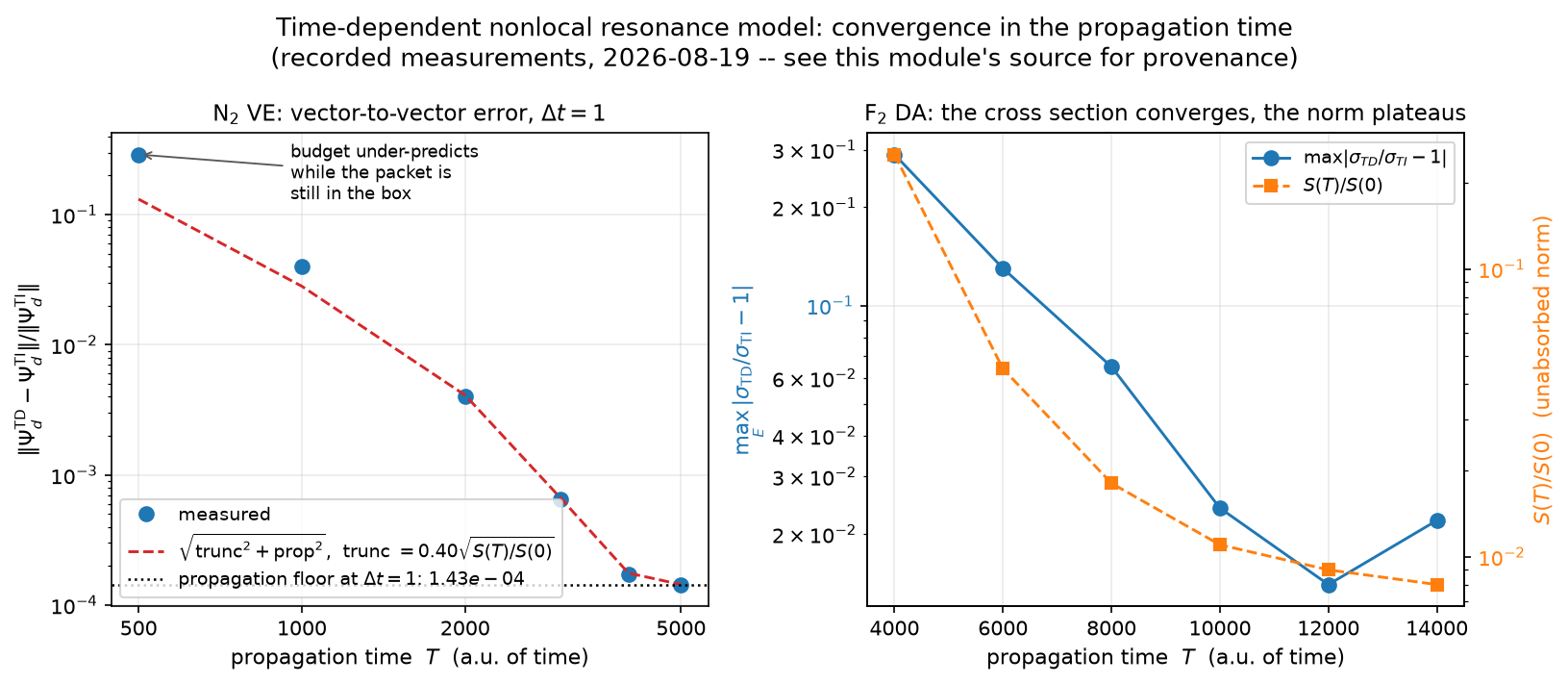
truncation(T) = 0.40 · sqrt(S(T)/S(0))        propagation(dt=1) = 1.43e-4
rel = sqrt(truncation² + propagation²)         (in quadrature, not linearly)

reproduces the convergence table to within 3% from T = 2000 onward (measured/budget 1.03, 1.03, 1.02, 1.00), which is what makes “this is convergence, not a bug” a demonstration rather than an argument.

It does not hold at short times — 2.2× at T = 500, 1.4× at T = 1000. The budget is asymptotic: truncation ∝ √(S(T)/S(0)) assumes the tail \(-i\int_T^\infty e^{iEt}\Psi(t)\,dt\) is dominated by a decaying remainder, and while the packet is still inside the box that premise does not apply. The shipped gate sits at T = 4000, well inside the regime where the budget is valid.

4. What the time domain shows that the resolvent cannot

4.1 The packet leaves — and on a coarse grid it does not

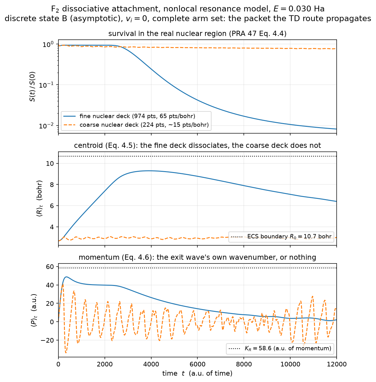
On F₂’s fine production nuclear deck (65 points/bohr over R = 3–10.7, largest node spacing 0.023 bohr) the DA packet dissociates: ⟨R⟩_t climbs monotonically 2.66 → 9.33 bohr, ⟨P⟩_t rises toward K_R ≈ 58, and S(t) falls 0.94 → 0.007 as the wave crosses the ECS absorber at R = 10.7.

⟨R⟩_t then turns over near t ≈ 4000 and falls back to ~6.4 bohr while ⟨P⟩_t decays toward zero. That is not the packet returning: it is the fast dissociating flux being absorbed at the boundary, leaving the bound remnant of §4.2 to dominate what is left inside the box. The turnover and the S(t) plateau are the same fact seen twice — which is also why ⟨P⟩_t peaks near 48 rather than reaching K_R = 58.6, since it averages the outgoing wave together with a slow bound population.

On a coarse deck it does none of this — the centroid creeps to 2.77 bohr and oscillates, survival plateaus at 0.673. The outgoing wavelength is 0.107 bohr against ~15 points/bohr, so the flux cannot propagate to the absorber and rattles in place. It looks bound and is not. Only the time-domain diagnostics distinguish the two; a resolvent returns a plausible number in both cases.

4.2 S(t) plateaus on F₂, and σ converges anyway

F₂’s V_d(R) has a well — minimum −0.149264 Ha at R = 3.363 against the F+F⁻ asymptote −0.126931, a depth of 0.0223 Ha — supporting ≥24 near-real modes with |Im E| = 1.5e-7 … 7.7e-6. The launch populates them with 5.08e-3 of its real-region norm, so S(t) flattens at 0.006–0.009 from T ≈ 12000 and no absolute survival floor is reachable on this molecule; removing their ≈2e-2 contribution to the transform would need T ≳ 1e7.

\(\sigma_\mathrm{DA}\) converges regardless, because it reads the wavefunction value at the outermost real node, where those well-localized modes have almost no amplitude. The observable converges while the norm does not, so convergence here is defined as \(\sigma_\mathrm{DA}\) stationary in T — not as S(T)/S(0) below a threshold. A convergence check written the obvious way would warn permanently on every F₂ run.

4.3 The launch basis, and what it says about the two discrete states

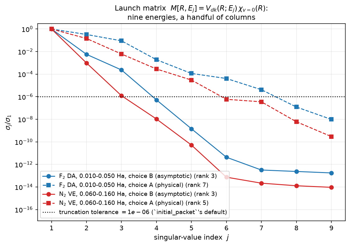
window	choice	σ₂/σ₁	σ₃/σ₁	σ₄/σ₁	rank @1e-6
F₂ DA, 0.010–0.050 Ha	B	5.7e-3	2.4e-4	5.3e-7	3
F₂ DA, 0.010–0.050 Ha	A	3.3e-1	9.0e-2	1.9e-3	7
N₂ VE, 0.060–0.160 Ha	B	9.8e-4	1.2e-6	1.1e-8	3
N₂ VE, 0.060–0.160 Ha	A	1.5e-1	6.2e-3	3.3e-4	5

PRA 47’s “single energy-independent wave packet” is essentially exact for choice B and materially approximate for choice A. The reason is structural: an R-independent \(\phi_d\) lets the launch state’s R-dependence enter only through \(\lambda(R)\), while choice A’s \(\phi_d(\cdot;R)\) injects genuine two-variable structure. This is an independent symptom of the same R-dependence that degrades choice A in the TI campaign (F₂ DA ratio 0.29–0.90; VE 0.565–1.140) and that PRA 77’s Sec. VI A predicts.

5. The arm set cannot be truncated

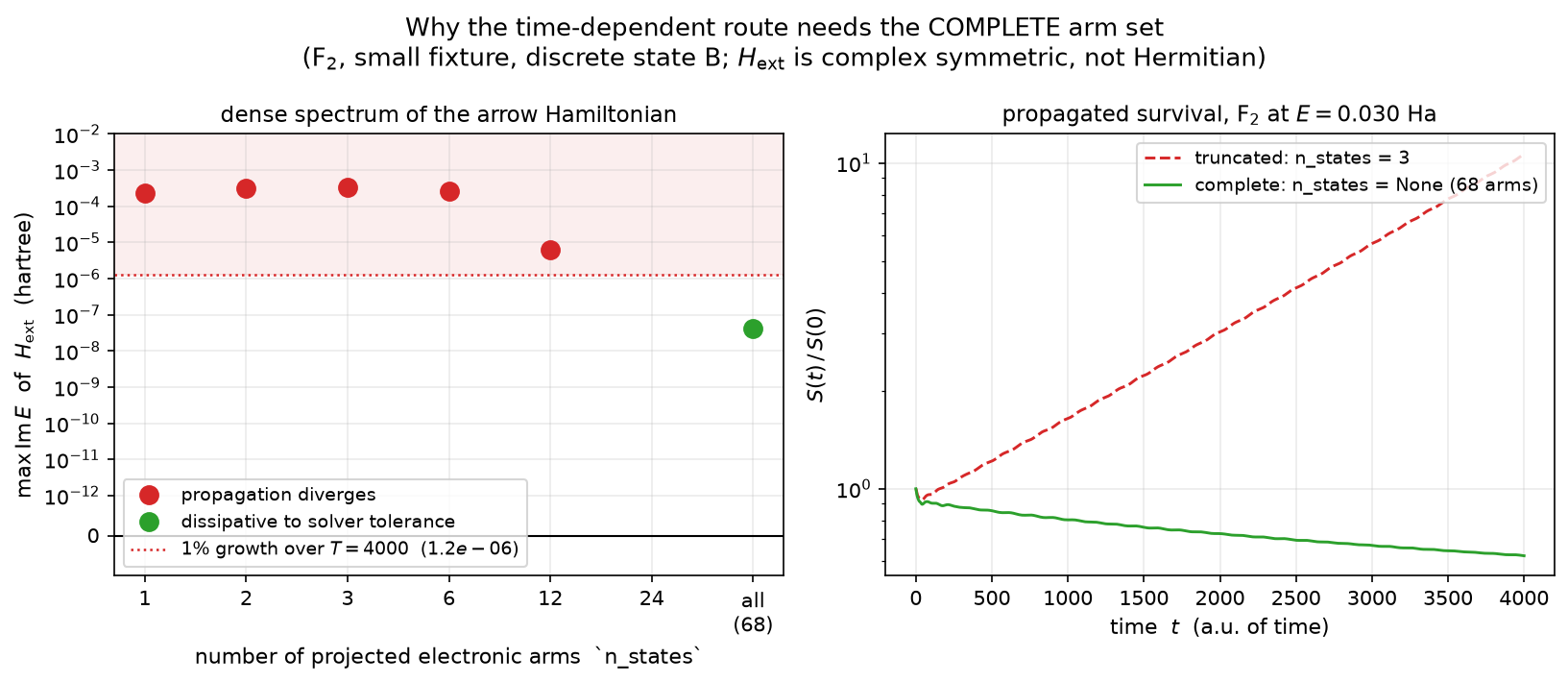
Truncating the sum over projected electronic states makes H_ext non-dissipative: modes acquire Im(E) > 0 and the propagation diverges exponentially in t. Dense eig gives max Im(E) = +2.787e-3 at n_states=3 on the N₂ gate deck and +5.84e-4 on the F₂ production fixture. That the divergence is identical to five digits across dt = 4/2/1/0.5/0.25 and Padé order 3 and 4 proves it is the operator, not the propagator.

The asymmetry with the time-independent route is the point. Truncating F(E) perturbs a resolvent by a bounded amount — which is why the TI campaign runs happily at _N_STATES = 100 — whereas a single eigenvalue crossing into the upper half-plane grows without bound in a propagator. The same approximation is benign in one route and fatal in the other, so the TI precedent does not transfer and an n_states convergence study is unavailable here.

The effect is non-monotonic — on one small F₂ fixture max Im(E) runs +1.60e-4 / +2.02e-4 / +1.96e-4 / +9.03e-6 at n_states = 1/2/3/8, then ≤0 from 12 onward, and +2.4e-12 for the complete set. So the rule is not “more arms is safer”: any truncation may leave growing modes, and establishing that a particular one does not requires a dense spectral check. n_states=None is the only value needing no check. propagate_nrm warns at runtime when a packet grows.

Spectral claims here require a dense eigensolver. These matrices are strongly non-normal and ARPACK eigs(which="LI") under-reports the largest imaginary part — +4.639e-4 against dense eig’s +2.787e-3 on the same 716-dimensional matrix, six times low. Sparse results are lower bounds.

The complete set’s own max Im(E) was an under-resolved ECS tail, and that is now settled. On three decks it sits at +1.4e-12 … +5.0e-13 — marginal stability, which is correct, since genuinely bound nuclear states do not decay (that is what §4.2 is). A small 68-arm F₂ fixture returned +6.98e-5 instead, five orders larger, while the propagation launched from \(\xi\) on that same fixture decayed. Neither of the two explanations first offered (a real but unpopulated mode; dense-eigensolver backward error) was right. Measured 2026-08-24 by refining that fixture’s nuclear ECS tail and nothing else:

nuclear tail elements (6 → 20 bohr)	complete set max Im(E)	Re E there	n_states=3 max Im(E)	Re E there
2	+6.98e-5	+958 Ha	+3.305e-4	−0.0754 Ha
4	+4.15e-8	+666 Ha	+3.305e-4	−0.0754 Ha
6	+4.71e-8	+4806 Ha	+3.305e-4	−0.0754 Ha

Two things separate at once. The complete set’s large value moves four orders under refinement and converges, and the eigenvalue carrying it sits at Re E of hundreds to thousands of hartree — a high-energy mode of the rotated continuum, at an energy the packet never occupies. It was a discretisation artifact of a tail spanning 14 bohr in two elements. The truncated set’s value does not move at all, on any tail, and sits at Re E = −0.0754 Ha, inside the packet’s own energy range. Artifact versus real growing mode is exactly this contrast, and it is why figure nrm-td-truncation-diverges.png classifies by a threshold rather than by the sign of Im E: the line it draws is where a mode would grow the packet by 1% over the propagation (ln 1.01 / 2T), which the truncations clear by four orders and the complete set misses by four.

Even so, a spectral argument is not what makes a propagation safe here — the runtime survival guard is. propagate_nrm’s check that the packet does not grow tests the thing that actually matters (is a growing mode populated?) rather than a sufficient condition on the operator, and it needs no dense eig at production size. Truncation is ruled out on both counts: the growing modes are real under refinement AND demonstrably populated — on this fixture S(t)/S(0) reaches 10 by T = 4000 at n_states = 3 while the complete set falls to ~0.6.

6. The Markovian limit — and which V_d it takes

PRA 47 Eq. (2.11): in the Markovian limit the memory kernel of Eq. (2.1) collapses to \(i[\Delta_L(R) - (i/2)\Gamma_L(R)]\,\delta(R-R')\,\delta(t)\), i.e. the local complex potential is the Markovian approximation to the nonlocal model. What remains is Eq. (2.15),

i ∂_t Ψ_d = [T_N + V_d(R) + Δ_L(R) − (i/2)Γ_L(R)] Ψ_d

with no arms at all, so the propagated matrix is N_R square — 974 on F₂’s production nuclear deck, against 53570 for the nonlocal one — and a converged run costs 4 s against ~30 min. td_nrm_da_cross_section(..., markovian=True, Vd=…, Gamma=…) selects it; nrm.extended.lcp_limit_hamiltonian and nrm.extended.lcp_initial_packet are the two pieces.

Everything measured in this section is reproduced end to end by

uv run --no-sync python -m validation.diatomic.td_nrm_figures markovian

(~9 min, almost all of it the two nonlocal propagations), which writes figures/nrm-td-markovian-vs-lcp.png and its .npz.

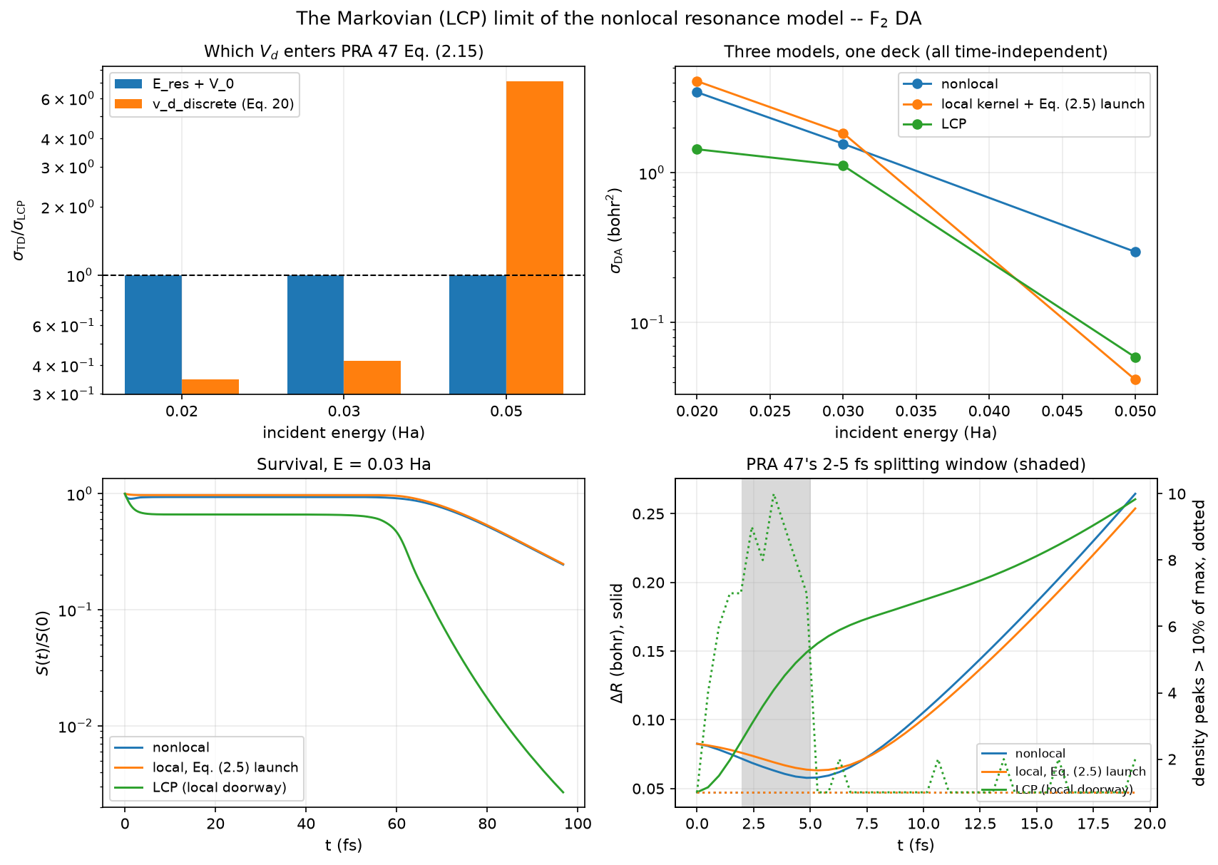
(In its lower-right panel the nonlocal peak-count trace lies exactly under the local one at 1 — that coincidence is §6.4’s result, not a missing curve.)

6.1 Which V_d enters Eq. (2.15) — measured, not argued

The repository has two candidates and they are not interchangeable: NrmIngredients.v_d_discrete (PRA 77 Eq. 20, \(V_0 + \langle\phi_d|H_\mathrm{el}|\phi_d\rangle\)) and qscat.core.lcp’s Vd (E_res(R), with V_0 already inside model.surface). Eq. (2.14), \(E_\mathrm{res} - V_d + V_0 - \Delta_L = 0\), rearranges to \(V_d + \Delta_L = E_\mathrm{res} + V_0\) — so Eq. (2.15)’s bracket is the second one, and the first is short by the level shift \(\Delta_L\). Both were run against the shipped lcp_da_cross_section on the F₂ fixture deck (dt = 2, T = 12000):

V_d in Eq. (2.15)	\(\sigma/\sigma_\mathrm{LCP}\) at E = 0.02	0.03	0.05 Ha
qscat.core.lcp’s Vd = E_res + V_0	1.000215	1.000198	0.999892
NrmIngredients.v_d_discrete (Eq. 20)	0.346	0.419	7.14

Decisive, and the failure of the second is not a normalization anyone could absorb — it changes sign of direction with energy. E_res + V_0 is what is shipped.

The difference between the two decays over the same R-range as \(\Gamma\) — measured on this deck:

R (bohr)	3.99	3.50	3.01	2.49	2.20	1.51
V_d(Eq.20) − V_d(LCP) (Ha)	2e-6	4.1e-5	9.5e-4	0.0423	0.268	1.171
\(\Gamma\) (Ha), frozen below R = 2.5033	0	0	0	0.0095*	0.0095*	0.0095*

It does not vanish wherever \(\Gamma\) does — R = 3.01 has \(\Gamma = 0\) and a difference of 9.5e-4 Ha, 500× the R = 3.99 value — and that is expected, not anomalous: \(\Gamma_L(R)\) is \(\Gamma\) at one energy while \(\Delta_L(R) = P\!\int (dE'/2\pi)\, \Gamma(E',R)/(E_\mathrm{res}-E')\) (Eq. 2.12a/2.13b) integrates \(\Gamma\) over all E′, so \(\Delta_L\) is free to be nonzero where \(\Gamma_L\) vanishes.

The starred \(\Gamma\) values are a frozen extrapolation, not F₂’s width. qscat.core.lcp.resonance_pole_walk freezes the last accepted \((\mathrm{shift},\ \Gamma)\) when the pole finder breaks down. On this reduced 55-point electronic deck it breaks at R = 2.5033 and holds \(\Gamma = 0.00949256\) over the inner 198 of 819 real nodes; the 132-point production deck runs on to R = 1.8657 and gives \(\Gamma\) = 0.0104 / 0.140 / 0.539 at R = 2.49 / 2.20 / 1.51 — 57× the frozen value at the innermost. The LCP doorway peak at R = 2.4864 is just inside the freeze, so on this deck the local kernel driving §6.3 and §6.4 is a frozen extrapolation across the whole region where the dynamics happen. Every comparison in §6 is differential — both sides consume the same curve — so no verdict here depends on it, but nothing in §6.3/§6.4 should be read as F₂’s converged physics. The walk now warns when it freezes.

6.1.1 “The doorway peak” names two different points

§4 of nonlocal-resonance-model.md records |V_d(Eq.20) − V_d(LCP)| = 0.0053 Ha for F₂ “at the doorway peak”, and §6.1 above reads 0.0423 Ha at “the doorway peak”. Both are right; the phrase is overloaded, and which point is worth a factor of 70 while the electronic deck is worth 1.3×:

| |V_d(Eq.20) − V_d(LCP)| at | reduced elec (55) | production elec (132) | |—|—|—| | \(\operatorname{argmax}\ \sqrt{\Gamma/2\pi}\cdot\lvert\chi_0\rvert\) — the LCP doorway (R = 2.486 / 2.478) | 0.04231 | 0.03283 | | \(\operatorname{argmax}\lvert\chi_0\rvert\) ≡ \(\operatorname{argmax}\lvert V_{dk}^+\chi_0\rvert\) — the NRM doorway, R = 2.745 | 0.00535 | 0.00534 |

The two points are 0.26 bohr apart, and over the region where \(\lvert\chi_0\rvert\) exceeds 5% of its maximum the difference sweeps 0.00095 → 0.067 Ha. §4’s number is the NRM doorway and is deck-stable to three significant figures; §6.1’s is the LCP doorway. Neither is a statement about \(\Delta_L\) being deck-sensitive — it is not.

6.2 The gate, and why it is tighter than the nonlocal one

\(\sigma_\mathrm{TD}/\sigma_\mathrm{LCP}\) = 1.000215 / 1.000198 / 0.999892 at E = 0.02/0.03/0.05 Ha. The residual is transform truncation and nothing else — dt = 1, 2 and 4 reproduce all three ratios to six digits, so the dt⁶ propagation error is far below it:

T	4000	8000	12000	16000	20000
max|ratio−1|	2.4e-2	1.3e-3	2.2e-4	3.6e-4	7.7e-5

The gate sits at 5e-3, an order tighter than the nonlocal route’s 5e-2, because there is no model difference in this comparison at all: same deck, same \((V_d, \Gamma)\), same Eq. (54) extraction, only the frequency-domain solve replaced by a propagation.

6.3 The doorway, not the kernel, is most of the LCP’s error on F₂

Eq. (2.11) localizes the kernel. Read strictly it leaves Eq. (2.5)’s launch state \(V_{dk_i}(R)\,\chi_v(R)\) alone, while the LCP this repository ships launches \(\sqrt{\Gamma_L(R)/2\pi}\,\chi_v(R)\) — \(\Gamma_L = \Gamma(E_\mathrm{res}(R), R)\), evaluated at the resonance position rather than the incident energy, and therefore energy-independent. Those are not the same vector: measured overlap 0.569, norm ratio 4.03. So there are three models, not two, and running all three on one deck separates what the kernel costs from what the doorway costs (TI values, \(\sigma_\mathrm{DA}\) in bohr²):

E (Ha)	nonlocal	local kernel + Eq. (2.5) launch	LCP (local kernel + local doorway)
0.02	3.443	4.082	1.433
0.03	1.559	1.837	1.116
0.05	0.296	0.0415	0.0586

All three are time-independent — the middle column is solve_nuclear with \(F \to \operatorname{diag}(-i\Gamma/2)\) and the Eq. (2.5) right-hand side, not a propagation. (Its TD counterpart reads 4.118 / 1.862 / 0.0423, i.e. 1.0087 / 1.0139 / 1.0188 of these — this route’s own transform-truncation offset at T = 12000, and the reason the columns must not be mixed.)

At 0.02 and 0.03 Ha, localizing the kernel alone moves \(\sigma\) by ~18–19% while the full LCP is off by 2.4× and 1.4× — i.e. most of the LCP’s error on F₂ comes from the local doorway, not from the Markovian kernel. At 0.05 Ha the ordering inverts and both approximations are wrong in different directions. This is a one-deck, one-molecule measurement on a reduced electronic grid, not a general claim.

What this is measured against matters. The reference column here is the nonlocal model, not the exact 2-D oracle, so strictly this decomposes the LCP’s error relative to the NRM. That is legitimate on F₂ only because NRM choice B tracks the exact oracle to 0.06–0.33% there (nonlocal-resonance-model.md §7.1) — on NO, where the NRM’s DA collapses by 5–8 orders (§7.2), the same decomposition would be measured against a broken reference and would mean nothing.

lcp_initial_packet implements the LCP doorway, because reproducing qscat.core.lcp is what markovian=True is for; the hybrid above is a measurement, not a shipped option.

6.4 The packet: no splitting on F₂

PRA 47’s mechanism for the H₂⁻ LCP failure is a temporary splitting of the nonlocal packet between ≈2 and ≈5 fs that a single complex curve cannot reproduce (p. 1041). On F₂ at E = 0.03 Ha, propagating the nonlocal and the local Hamiltonians from the same Eq. (2.5) launch state — the comparison that isolates the kernel — there is no such thing:

t (fs)	0	2.4	2.9	3.4	3.9	4.8	6.8	9.7
nonlocal, density peaks >10% of max	1	1	1	1	1	1	1	1
local, density peaks >10% of max	1	1	1	1	1	1	1	1
nonlocal, \(\Delta R\) (bohr)	0.083	0.069	0.066	0.063	0.061	0.058	0.066	0.101
local, \(\Delta R\) (bohr)	0.083	0.074	0.072	0.069	0.067	0.064	0.067	0.096

Two different weightings are in play here and only one is right for each row. The peak count is taken on the density in wavefunction-value space (\(\lvert\psi_i\rvert^2 = \lvert c_i\rvert^2/w_i\)), which is what a shape looks like on a non-uniform grid — counting peaks in coefficient space would find element boundaries. \(\Delta R\) is √(⟨R²⟩−⟨R⟩²) on the probability density in DVR coefficient space, where |c_i|² already carries the quadrature weight, the same convention propagation._record uses for ⟨R⟩ and ⟨P⟩; taking that moment in value space instead drops w_i from the integrand and produces a different and inverted trend (an earlier draft of this table did exactly that).

Both stay unimodal, and both contract monotonically to ≈4.8 fs before re-expanding — one breathing packet, not two, and the nonlocal and local widths never differ by more than 0.007 bohr. Over the full run the two are nearly indistinguishable in the Eq. (4.5)/(4.6) moments — ⟨R⟩ agrees to ≤0.01 bohr and ⟨P⟩ to ≤0.15 a.u. at every sample through T = 4000 — and differ only in an early, one-off norm loss: S(t)/S(0) plateaus at 0.9368 for the nonlocal against 0.9733 for the local, the whole gap opening inside the first ~4 fs and nothing changing after.

The shipped LCP’s packet does look different — S/S₀ drops to 0.663 at once, ⟨P⟩ runs ~55 against ~40, and it reaches the absorber ~10 fs earlier — but that is the doorway of §6.3, not the kernel.

And it is not unimodal: 9 / 8 / 10 / 9 / 7 peaks at t = 2.4 / 2.9 / 3.4 / 3.9 / 4.8 fs, collapsing back to 1 by 6.8 fs, with \(\Delta R\) climbing monotonically 0.047 → 0.185 bohr. The claim above is about the nonlocal and Markovian packets only, not about this one. This transient structure is almost certainly the launch state ringing off the step in \(\sqrt{\Gamma}\) at §6.1’s freeze boundary (R = 2.5033, essentially on top of the LCP doorway peak at 2.4864), not a physical splitting — it is a reason to distrust that packet on this deck, not evidence for PRA 47’s mechanism.

This is a negative result about F₂, not about PRA 47. F₂ is the molecule where the nonlocal model reproduces the exact oracle to 0.06–0.33% (nonlocal-resonance-model.md §7.1); a mechanism the paper found in a system whose LCP fails by 14× is not expected to show up here, and the honest reading is that F₂ is a poor place to look for it.

7. Vibrational excitation

td_nrm_ve_cross_section is the second consumer of the same \(\Psi_d\), and all of it is a contraction. T^res is vibrational_excitation.t_resonant(\(\chi_f, V_{dk_f}^+, \Psi_d\)) and T^bg is t_background, both called unchanged, so PRA 77 Eq. (34)/(35)’s non-conjugated V⁺_dk and Eq. (37)’s \(\phi^+\) at the final channel energy are inherited from the time-independent route rather than re-derived. T^bg contains no \(\Psi_d\) at all — it is energy-domain and static — so it is bit-identical between the two routes. That is what makes running both include_background settings a diagnostic rather than a duplicate: a discrepancy appearing only with the background could not be a background error, it would mean the resonant term is being combined with it wrongly.

One propagation serves every energy and every final channel: H_ext is energy-independent (§2.4) and \(\Psi_d^+\) does not depend on v'.

7.1 VE converges long before DA does, and the observable is why

T^res weights \(\Psi_d\) by \(\chi_f\), which lives in the interaction region, so the transform converges once the amplitude there has decayed — whether by autodetachment or by simply moving outward. \(\sigma_\mathrm{DA}\) reads the wavefunction value at the outermost real node, so its packet has to cross the whole box first (§4.1). The clean measurement is F₂, where both observables run on one deck, from one propagation:

deck	observable	dt	T	max|σ_TD/σ_TI − 1|
F₂, 974 nuclear × 55 electronic	VE, 0.03/0.05 Ha, v’ = 0/1	2	2000	9.8e-5 (5.9e-5 with background)
F₂, same deck	DA, 0.02/0.03/0.05 Ha	2	4000	0.29
F₂, same deck	DA, same energies	2	12000	1.4e-2
N₂, 179 nuclear × 74 electronic	VE, 0.06/0.10/0.15 Ha, v’ = 0/1	1	4000	2.7e-4 (a null — below)

VE is converged at a sixth of DA’s T, on the same packet, while 93.8% of it is still in the real region. Nothing has left; what decayed is the amplitude under \(\chi_f\). A molecule whose DA channel is open therefore does not pay the DA cost for a VE observable.

7.1.1 Both residuals have an oscillatory floor — and sampling T coarsely hides it

Neither molecule converges monotonically to round-off, and neither single number above should be quoted as “the accuracy”. §4.2’s long-lived components of \(\Psi_d\) — anything under \(\chi_f\) that does not decay within the propagation — each contribute a term that oscillates in T instead of decaying. Where a given run lands on that oscillation is a matter of phase.

N₂, dt = 1, worst of six channels. Coarse sampling looks like clean convergence (4.2e-1 → 5.0e-2 → 2.7e-4 at T = 1000/2000/4000, and the same to one figure without the background). A fine scan says otherwise:

T	3600	3640	3680	3720	3760	3800	3840	3880	3920	3960	4000
max|ratio − 1|	2.43e-3	1.21e-3	1.01e-3	1.15e-3	1.96e-3	2.40e-3	2.45e-3	2.15e-3	1.60e-3	9.11e-4	2.71e-4

The E = 0.06, v’ = 1 channel traces a clean sinusoid (1.002433 → 0.997553 → 0.999793) of period ≈450–500 a.u. and amplitude ≈2.4e-3 which crosses 1 almost exactly at T = 4000. The honest N₂ statement is an envelope, ≤2.5e-3, and the shipped gate is 5e-3 — twice it. (A 1e-3 gate passes at T = 4000 and fails by 2.4× at T = 3800; the T = 3800 point was re-run independently and reads 2.399e-3.) The T = 4000 value coinciding with the vector-to-vector identity gate’s 1.73e-4 (§3) is likewise a coincidence of phase, not a confirmation.

F₂, dt = 2, worst of four channels. Where its gate operates the residual is a plateau, not a phase:

T	1600	1680	1760	1840	1920	2000	2080	2160	2240	2320	2400
max|ratio − 1|	7.21e-5	7.04e-5	6.31e-5	6.34e-5	5.98e-5	5.95e-5	6.61e-5	6.70e-5	5.75e-5	4.88e-5	7.47e-5

and all four channel ratios carry the same sign there (+3e-5 … +7e-5) — a systematic discretisation offset, not a zero crossing. F₂’s oscillation starts later and grows: 1.9e-4 (T = 2800), 3.2e-4 (3000), 9.6e-4 (3400), 1.5e-3 (3800), 2.5e-3 (4000). So the shipped F₂ gate is 1e-3, 10× the worst of the two include_background settings it asserts (9.8e-5; the T scan above is the include_background=True curve, whose plateau is 5.9e-5 and 17× under the gate). Either way the gate is sized to the plateau it actually runs on, rather than to a multiple of an envelope the test never reaches.

The general lesson is the one this section exists for: a T-convergence claim from three sampled points is not a convergence claim. Sample finely enough to see the period, then gate on the envelope if you are on one and on the plateau if you are on that.

7.1.2 dt = 1 on N₂, dt = 2 on F₂

The N₂ deck’s dt = 2 residual is 1.52e-2 at T = 4000 and flat at that value across T = 3000–4000 — an order above the dt = 1 envelope and not oscillating, i.e. a genuine propagation error rather than a phase. dt = 2 is inadequate there. Do not read 1.52e-2 / 2.71e-4 = 56 as dt⁶’s predicted 64 confirmed: the denominator is the null of §7.1.1, and the agreement is arithmetic on a coincidence. Neither F₂ run needs the correction — the DA gate’s truncation floor is 1.4e-2, two orders above its own propagation error, and the VE run’s total dt = 2 error is 5.9e-5 on the plateau, which bounds its propagation term below that.

7.2 The Markovian VE limit substitutes the doorway at BOTH ends

Eq. (2.11) localizes the kernel; §6.3’s point was that the shipped LCP also replaces the doorway. For VE that doorway appears twice — as the launch state and as the coupling the exit channel is contracted against — and markovian=True replaces both with \(\sqrt{\Gamma_L/2\pi}\), which is exactly the \(S_{v' \leftarrow v} = \langle \sqrt{\Gamma_L/2\pi}\cdot\chi_{v'} | \Psi_d \rangle\) the repository’s own LCP VE route (qscat.core.lcp.lcp_ve_cross_section) computes. Keeping the nonlocal V⁺_dk_f at the exit while localizing the kernel would be a third model, so it is not offered. include_background=True is refused with markovian=True for the same reason: Eq. (37)’s background is built from \(\phi_d\) and the P-space scattering states, which the local model does not have.

Measured against a reference assembled in-test from solve_nuclear + t_resonant (libs/qscat may not import projects); that assembly is term-for-term qscat.core.lcp.lcp_ve_cross_section’s doorway, H_res and S, and the test records the shipped route agreeing to twelve digits on the F₂ fixture deck of §6 (dt = 2, v = 0, E = 0.02/0.03/0.05 Ha, v’ = 0/1):

T	2000	4000	12000
max|σ_TD/σ_LCP − 1|	5.6e-6	3.3e-6	4.3e-6

The gate sits at 5e-5, 8.9× the worst residual in that range (5.6e-6, not the 3.3e-6 at the test’s own T).

Converged by T = 2000 and flat thereafter — on the same deck whose DA Markovian comparison needed T = 12000 to reach 2.2e-4 (§6.2). Same model, same packet, same propagation, two observables: §7.1’s argument with every model difference removed.

7.3 The unabsorbed warning is a DA criterion, and it over-warns on VE

td_nrm_ve_cross_section applies the same unabsorbed/S(0) > 1e-2 test td_nrm_da_cross_section uses, and on VE it fires while the cross section is already converged — F₂ at T = 2000 warns at 0.938 and is right to 6e-5. Read it as what it says, “the packet is still in the box”; it is not evidence that \(\sigma_\mathrm{VE}\) is wrong. Convergence here is \(\sigma_\mathrm{VE}\) stationary in T, exactly as in §4.2. The threshold is not retuned for VE: a warning that is conservative for one observable and calibrated for the other is better than two thresholds, and _UNABSORBED_TOL’s calibration is a DA measurement (td_cross_section.py).

8. What the kernel is doing while it runs

The resolvent route returns \(\Psi_d(R;E)\) and nothing about how it was reached. The extended-space propagation of §2.2 carries one auxiliary nuclear packet \(\varphi_n\) per projected electronic state, and those packets are the memory: PRA 77 Eq. (55)’s kernel \(F(E)\) is what you get by eliminating them. So they can be watched, and qscat.core.nrm.memory watches them.

Three series, recorded during the same propagation that produces the cross section, at a cost measured identical to not recording them:

\[ A(t) = \sum_n \lVert\varphi_n(t)\rVert^2 , \qquad X(t) = 2\,\mathrm{Im}\,\langle \Psi_d(t) | \textstyle\sum_n V_{dn}\varphi_n(t)\rangle , \]

\[ X_{\mathrm{loc}}(t) = -\langle \Psi_d(t) | \Gamma_{\mathrm{loc}} | \Psi_d(t)\rangle . \]

\(A\) is arm_norm (with arm_norm_by_channel and arm_peak resolving it by block), \(X\) is exchange — the rate at which the arms feed the discrete state — and \(X_{\mathrm{loc}}\) is exchange_local, the same rate in the Markovian limit, with \(\Gamma_{\mathrm{loc}}\) read off the kernel itself by local_width, \(\Gamma_{\mathrm{loc}}(R_i) = -2\,\mathrm{Im}[(F\sqrt{w})_i/\sqrt{w_i}]\).

The comparison \(X\) against \(X_{\mathrm{loc}}\) is the point. \(X_{\mathrm{loc}}\) is non-positive wherever \(\Gamma_{\mathrm{loc}} \ge 0\): a local model can only drain the discrete state. \(X > 0\) is amplitude coming back, which the LCP cannot represent at all.

That condition is not free, and local_width deliberately does not clamp: \(\Gamma_{\mathrm{loc}}\) is a width only where the channel is open, and outside that window it decays to round-off and comes back signed either way — 32 of N₂’s 179 nodes are negative at \(-3.8\times10^{-9}\) against a peak of \(2.5\times10^{-2}\). Not clamping is what keeps that visible. test_the_markovian_limit_can_only_lose gates \(X_{\mathrm{loc}} \le 0\) on a real deck rather than in the algebra, but it gates N₂ only; the campaign measured it strictly negative on all three, and F₂ is the one to watch, since its packet dissociates into exactly the region where \(\Gamma_{\mathrm{loc}}\) is round-off-signed.

Every number below carries its normalization in its name, because the two in use differ by orders: on the N₂ gate deck a raw positive maximum of \(+8.776\times10^{-7}\) is \(+2.420\times10^{-4}\) divided by \(S_d(0)\) and \(+1.64\times10^{-3}\) divided by \(S_d(t)\).

8.1 arm_norm is not a population

Under ECS \(H_{\mathrm{ext}}\) is complex symmetric, so no conjugating norm is conserved and \(A\) is not a probability that \(\lVert\Psi_d\rVert^2\) gives up. The size of that gap is measured rather than assumed: imbalance compares the coupling’s two one-sided rates, and their difference is a median 0.822 of the larger on the gate deck — the same size as the transfer, not a correction to it. Per molecule the medians are 0.871 (N₂), 0.938 (NO), 0.080 (F₂).

arm_norm is therefore a relative channel decomposition: read across channels, and against itself over time. The figure’s partition curves do not sum to anything conserved and are not drawn as if they did.

arm_peak ranks the blocks by their own maximum, which is what a truncation would have to respect. It does not favour low indices: the four largest blocks are 3, 4, 2, 5 on N₂, 2, 3, 4, 1 on F₂ and 1, 0, 2, 3 on NO. The percentages beside them in the driver — 33.7 %, 47.3 %, 89.6 % — are arm_first_four_share, the share carried by blocks 0–3, which is what a positional truncation would actually keep; the two sets coincide only on NO. Keeping “the first few” arms would be wrong on two of the three — a second, independent reason for n_states=None beyond §5’s.

8.2 The campaign

Three molecules on their existing gate decks, each on the electronic box its own E_BOX_LADDER rung converges at (N₂ \(r_{\max}=16\), NO 16, F₂ 20), n_states=None, order-3 Padé at \(dt = 1\) to \(T = 4000\).

That ladder converges \(\Gamma_{\mathrm{loc}}\), not the observables below. It is the right criterion for exchange_local, which divides the run by that array, and it is not a convergence study of nonlocality or of the returning flux in the electronic box — no such study has been run. N₂ is the case to be careful with: 16 is the only rung where the adiabatic tracking is usable (min_overlap 0.820, against 0.374 / 0.216 / 0.015 at 14 / 20 / 24), so N₂’s per-block numbers in §8.1 rest on a box with no converged neighbour to check them against.

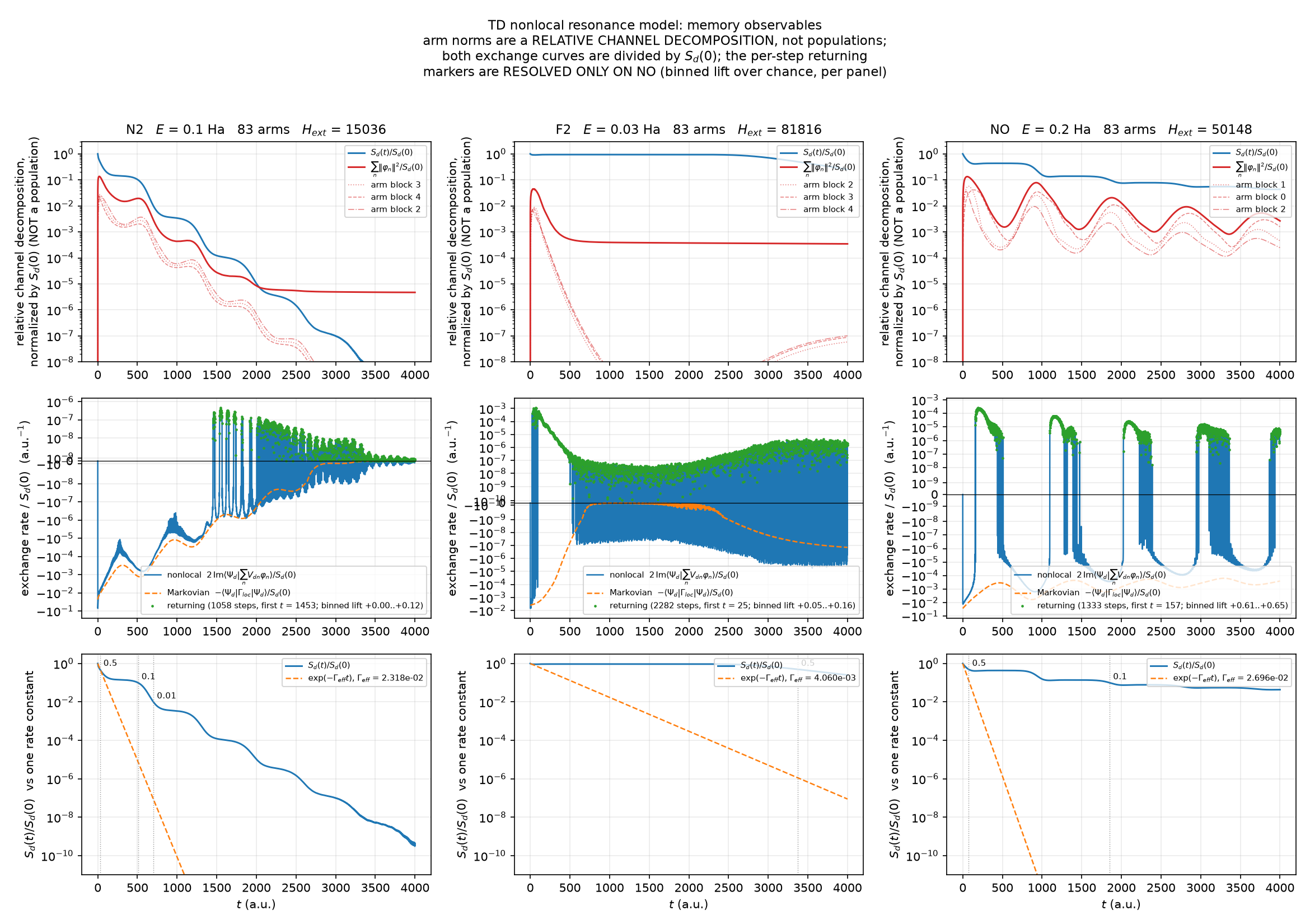
	N₂	NO	F₂
\(E\) (Ha)	0.100	0.200	0.030
\(N_R\) (real) / arms / \(H_{\mathrm{ext}}\)	179 (153) / 83 / 15036	597 (507) / 83 / 50148	974 (819) / 83 / 81816
peak RSS	0.76 GB	3.4 GB	5.82 GB
\(S_d(0)\)	3.482e−3	3.879e−3	5.203e−4
\(\Gamma_{\mathrm{eff}}\) (a.u.)	2.318e−2	2.696e−2	4.060e−3
arm peak / \(S_d(0)\), at \(t\)	0.1364 at 18	0.1334 at 55	0.0451 at 40
max positive / own peak \(\lvert X\rvert\)	6.402e−6	1.982e−2	1.590e−1
first return at \(t\)	1453	157	25
\(S_d/S_d(0)\) there	0.000	0.411	0.918
nonlocality	0.507	0.813	0.946
\(S/S_0 = 0.5\) at \(t\)	28	75	3371
…over \(\exp(-\Gamma_{\mathrm{eff}}t)\)	0.947	3.76	4.393e5
imbalance, median	0.871	0.938	0.080

Every row is that molecule at that energy. All of them except nonlocality are energy-independent (§8.4), so only that row needs the qualifier — and it needs it: these three energies are all inside the window where §8.4 finds the observable valid, but nonlocality does move with energy and inflates near a threshold.

The whole thing fits on a laptop. F₂ is the largest at \(H_{\mathrm{ext}} = 81816\) and peaks at 5.82 GB. An earlier note in this repository stated that 53570 “does not fit on a laptop” on the strength of three OS kills; those kills were concurrency, not size, and that claim is withdrawn.

8.3 The returning flux: what it shows, and where it cannot be read

At their campaign energies the nonlocality integral \(\int\lvert X - X_{\mathrm{loc}}\rvert \,/\, \int\lvert X_{\mathrm{loc}}\rvert\) reads N₂ 0.507, NO 0.813, F₂ 0.946, and every return-flux comparator in the table ranks the three the same way. That ordering is what this sub-project set out to establish, and only one of the two columns turned out able to carry it. Separating them took most of the work.

The pointwise sign of \(X\) is not a converged quantity on any of the three. Halving \(dt\) does not lengthen the sign-flip period in atomic units — it shrinks it, so the period stays at roughly two steps whatever the step is: F₂ \(2.09 \to 0.84 \to 0.52\) a.u. at \(dt = 1 / 0.5 / 0.25\), N₂ \(7.33 \to 1.34 \to 0.72\), NO \(34.5 \to 3.19\). A structure that sits at the step scale at every step size is being measured at the wrong resolution.

Those periods, and the per-refinement nonlocality spreads quoted below, come from the refinement runs recorded in N2_RESOLUTION and re-measured 2026-08-28 on sadaharu (x86, MUMPS) against the committed campaign .npz; the driver reprints both from the .npz under resolution --against <molecule>.

That this is time discretisation and nothing else was checked rather than assumed. Each campaign deck was re-propagated on a different CPU, BLAS and sparse factorisation (x86 + MUMPS against arm64 + SuperLU): the runs agree to 1.9e−13 (N₂), 1.3e−12 (NO), 8.4e−13 (F₂) with 100 % sign agreement.

So the returns are compared on time-averaged bins, at four widths (5, 10, 20, 50 a.u.) so that the width cannot be doing the work, against every refinement available per molecule. Two columns are read, because agreeing about the sign of a bin says nothing about its size:

	N₂	F₂	NO
lift of returning bins over chance	0.000–0.122	0.048–0.162	0.613–0.650
median magnitude disagreement there	125–148 %	84–520 %	2–19 %
max positive / own returning-window floor	0.07, 0.17	0.65, 1.02	2.23, 2.58

Lift, not raw concordance. The concordance is conditional — “of the bins this run calls returning, how many does the finer one?” — so its null is the finer run’s own positive-bin rate, not one half. That rate is ~0.59 on F₂ and ~0.35 on NO, so raw numbers of 0.65 and 0.98 mean opposite things. An earlier reading of this table quoted the raw values and put F₂ in a middle band; that band was the missing null, not a finding.

So there are two bands, not three, and the magnitude row is what settles it, because it involves no choice of metric: NO’s binned returns agree to 2–19 % where N₂’s and F₂’s differ by more than they are worth. N₂ and F₂ are not ranked against each other here — their lifts are both small and positive, and which of the two looks larger depends on whether the comparison is pointwise or binned (it reverses). One molecule of three carries a readable returning flux; the other two are not ordered by this observable.

This retracts a claim this sub-project made. The design document’s headline returning flux does not hold on N₂, and does not hold on F₂ either. N₂’s lift is zero at three of four widths and its binned returns differ in size by more than they are; the physics agrees with the arithmetic, since N₂’s first return is at \(t = 1453\), by which time \(S_d/S_d(0)\) has fallen below \(10^{-3}\) (the table’s cell rounds to 0.000) and there is nothing left to return to. The prototype’s \(+8.776\times10^{-7}\) is withdrawn twice over: it is below this floor, and it was measured on an \(r_{\max} = 11\) box that E_BOX_LADDER shows is 22 % wrong in \(\Gamma_{\mathrm{loc}}\) before resolution is considered.

The bin metric was introduced after the pointwise one failed, which is how a claim gets rescued rather than tested. Note which way it cut: it did not raise N₂, and once its null was supplied it removed F₂ as well.

So the returning flux cannot carry a comparison between molecules, being readable on one of them. nonlocality can be measured on all three and converges under refinement — N₂ 0.5068–0.5097 over four runs (0.6 %), NO 0.8131–0.8134 (0.04 %), F₂ 0.9398–0.9576 (1.9 %) — so the ordering is read off it instead. §8.4 is what qualifies that, since converging under refinement and being meaningful at a given energy are different things.

8.4 The ordering, and the window it is measured over

The three molecules run at three different energies, each set by where that molecule’s channel is open. So the comparison across them has to survive the possibility that it is a comparison in energy. All three were laddered — seventeen rungs — with everything else held fixed.

Every column the campaign reads as a return is frozen. Over a 4–6× change in \(\Gamma_{\mathrm{eff}}\) the onset does not move at all and max positive / peak moves in the fifth figure. Those are properties of the molecule.

nonlocality is not frozen, and over the full run it is not even the right integral. With the arms empty \(X = 0\), so \(\lvert X - X_{\mathrm{loc}}\rvert = \lvert X_{\mathrm{loc}}\rvert\) identically and the ratio is pinned near 1 whatever the kernel is doing. Every propagation passes through that window. Near a threshold it dominates, because the denominator collapses: \(\int\lvert X_{\mathrm{loc}}\rvert\) falls 46× across N₂’s ladder and 35× across F₂’s, while the numerator cannot fall below that floor.

What collapses is \(\Gamma_{\mathrm{loc}}\)’s magnitude over the doorway — \(\max \Gamma_{\mathrm{loc}}\) moves 5.5× on N₂ and 11.8× on F₂ — not its extent: the nodes carrying it go only 89 → 95 of 153 on N₂ and 291 → 360 of 819 on F₂. The reference dies in size, not in reach.

The contamination is a window, so the fix is a window. Integrating from the arm-norm peak onwards (nonlocality_post_peak) removes it from every rung, rather than discarding whole propagations for containing it. \(t_{\mathrm{peak}}\) is not a tuned knob — it is identical at every energy within a molecule (18 / 55 / 40 a.u.), and starting at \(2t\) or \(3t\) gives the same verdict.

The only rungs excluded are the two this ladder added outside the molecules’ own declared energy windows — N₂ at 0.05 Ha and NO at 0.40 Ha — by a criterion this module has carried since before the ladder existed, applied to both.

	N₂	NO	F₂
in-window rungs	6	4	5
nonlocality (post-peak)	0.224–0.773	0.870–0.872	1.055–1.341
margin to the next band	—	+12.5 %	+21.0 %

N₂ < NO < F₂. Of the three inequalities, NO < F₂ is the one to quote if only one can be: it holds on the raw full-run column too, over all seventeen rungs (NO’s max 0.8134 against F₂’s min 0.9246), needing no argument about windows at all. N₂ < F₂ holds with a wide margin. N₂ < NO is the narrowest at 12.5 % and the first to re-examine.

An honesty note, because this section has said three different things. It first reported the ordering, then retracted it outright, and now states it again on a different integral. The retraction was made on the full-run column with near-threshold rungs in it and was an over-reaction to a real problem. The first repair excluded four rungs by a share cut invented after the ladder was run — better, but open to the charge that a criterion had been fitted to the answer, and it could not support N₂ < NO at all, since N₂’s in-window 0.06 Ha rung read 0.848 there, above NO. Integrating post-peak removes the contaminated window instead of the contaminated rungs; that rung reads 0.416 post-peak, and no after-the-fact criterion remains.

8.5 What does not follow, and one negative result

NO’s flatness is not a measurement. Its nonlocality varies by 0.3 % over its entire declared window — but so does everything feeding it: \(\Gamma_{\mathrm{eff}}\) spans 1.02× and \(\int\lvert X_{\mathrm{loc}}\rvert\) 1.06×, against 4–6× and 35–46× on the other two. The perturbation that moved N₂ and F₂ was never applied to NO. “NO’s memory is energy-independent” would be reading an output that did not move under an input that did not move either; the honest statement is that NO’s Markovian reference does not vary on this deck, so its nonlocality has no energy dependence available to show.

NO’s returning flux is resolved, and it is the only one that is. Its returns come in periodic bursts, begin at \(t = 157\) with the discrete state still 41 % intact, reproduce at a lift of +0.61 to +0.65 over chance, and agree in magnitude to 2–19 %. Bursts on that timescale are what boomerang recurrences look like in the memory kernel — the packet re-entering the autodetachment region on each swing. That is a connection to the published interpretation of NO’s long-lived structure, not a new claim about it.

N₂ and F₂ are not ranked against each other by the returning flux. Both lifts are small and positive, and which looks larger reverses between the pointwise and binned metrics. Only the ordering on nonlocality above is claimed.

9. Limits — what this does not establish

• The TD/TI agreement validates the propagation, not the model. Both routes run on the same grids with the same ingredients, so shared discretisation error cancels. Absolute scale is anchored elsewhere (validation/n2/exact2d.py against Houfek at GATED_RTOL=1e-3).

• DA is F₂ only. NO’s DA channel is a known open failure for the TI route (docs/physics/nonlocal-resonance-model.md §7.2), so a TD run there would be measuring an already-broken oracle.

• The DA fixture uses a reduced 55-point electronic grid. The TD/TI ratio is insensitive to it (3–4 significant figures), but the fixture’s absolute \(\sigma_\mathrm{TI}\) is not the converged F₂ cross section.

• No production-electronic-deck data point exists on any molecule yet.

• VE is N₂ and F₂, choice B, 0→0 and 0→1. NO is not run — its time-INDEPENDENT VE is not run either (nrm-vibrational-excitation.md §5) — no higher final channel is, and choice A is not: every VE number here is AsymptoticDiscreteState.

• The VE agreement is differential, like every other number in this note. It says the propagation reproduces the resolvent on one deck; how well the nonlocal model reproduces the exact VE cross section is nrm-vibrational-excitation.md §4’s measurement (better than 0.7%), not this one’s.

• §6’s packet comparison is F₂ at one energy on the reduced electronic deck. It says what the Markovian collapse does there; PRA 47’s H₂⁻ is a different molecule with a 14× LCP failure, and nothing here contradicts or reproduces it.

• The Markovian gate validates the propagation, not the LCP. It shows the time-domain and frequency-domain routes to qscat.core.lcp’s own model agree; how good that model is remains docs/physics/nonlocal-resonance-model.md’s question.

• §8’s observables are diagnostics of a model already gated, not evidence for it. Every §8 number is read off a propagation whose cross section is validated in §3 and §7; none of them validates anything in turn. A molecule scoring high in nonlocality is a statement about this model’s kernel, not a measurement of how wrong the LCP is on that molecule.

• §8’s ordering is read from the post-peak integral over each molecule’s declared energy window, not from the full-run integral, and two of the seventeen rungs are excluded for falling outside those windows. NO < F₂ needs neither and holds on the raw column; the other two inequalities do.

• N₂ < NO rests on a 12.5 % margin between six N₂ rungs and four NO ones. It is the first of the three to fail if any does.

• nonlocality is a function of energy as well as molecule. A single value quoted without an energy means nothing, and over the full run it inflates near a threshold because its Markovian reference collapses in magnitude rather than because the kernel is more nonlocal.

• NO’s flat nonlocality is not evidence of anything: its \(\Gamma_{\mathrm{eff}}\) and Markovian reference are flat across its whole declared window too, so the perturbation was never applied.

• The returning flux is readable only on NO. Read against their own nulls, N₂’s and F₂’s binned returns lift 0.00–0.12 and 0.05–0.16 over chance and their magnitudes differ by 125–148 % and 84–520 %; neither is quoted as a measurement, and the two are not ranked against each other.

• NO’s own LCP remains undetermined, and §8 does not fix it. Its pole walk still does not converge in the electronic box; §8 ranks NO by a route that never calls the pole walk, which is a way around that failure and not a repair of it.

• O₂ is absent by choice. qscat.model registers O2, O2_SO12 and O2_SO32, but those are the potential factory’s fit rather than a published parameter set, so there is no external LCP comparison and §8’s comparative question is undefined for them.

10. Literature

• PRA 47, 1031 (1993) — reference/literature/gertitschke-1993-pra47-1031.md. The time-dependent nonlocal equation of motion Eq. (2.1)–(2.5), the amplitude transforms Eq. (2.6)/(2.8)/(2.9), the LCP limit in the time domain Eq. (2.11)–(2.15), and the packet diagnostics Eq. (4.4)–(4.6).

• PRA 77, 012710 (2008) — reference/literature/houfek-2008-pra77-012710.md. The model: Eq. (52), Eq. (60)–(61), Eq. (31)/(37)/(38), Eq. (54).

• PRA 95, 022714 (2017) — reference/literature/vana-houfek-2017-pra95-022714.md. What time-dependent formulations of these models are for, and the closing proposal this sub-project executes (p. 022714-16).

• PRE 75, 036707 (2007) — reference/literature/vandijk-2007-pre75-036707.md. The diagonal-Padé propagator.