NRM vibrational excitation¶
Location: qscat.core.nrm.vibrational_excitation (j_dk, t_resonant,
t_background, nrm_ve_cross_section) and qscat.core.nrm.scattering
(scattering_state_minus); libs/qscat/tests/test_nrm_ve.py,
test_nrm_scattering.py; validation/diatomic/ve_nrm.py + test_ve_nrm.py +
ve_nrm_figure.py; apps/qscat-run’s nrm method on a ve observable.
Source: K. Houfek, T. N. Rescigno, C. W. McCurdy, Phys. Rev. A 77,
012710 (2008) — reference/literature/houfek-2008-pra77-012710.md. Split out
of nonlocal-resonance-model.md, which holds
the method core (the kernel \(F(E)\), the discrete-state choices, the
ingredients) and the dissociative-attachment side; this note’s §1–§10 were
that note’s §8.1–§8.10.
Units: atomic units throughout (hartree, bohr).
Key result¶
Vibrational excitation is the channel PRA 77 plots for every molecule in
its study, so it is where the nonlocal model can be checked against the
exact solver most broadly — and choice B plus the background term
reproduces the exact driven.ve_cross_section oracle to better than 0.7%
on both N₂ (11 energies, 0.06–0.16 Ha) and F₂ (6 energies, 0.02–0.09 Ha),
elastic and first-inelastic alike (worst ratio 0.99623–1.00692 over all
four molecule/transition pairs), while choice A degrades to 0.565–1.140.
The reason B is that good is physics, not luck: an R-independent
\(\phi_d\) carries no derivative couplings, so the model is formally exact
and the residual is discretization error. The comparison is differential
(both routes on the same grids): it validates the model reduction, not
the grid.
1. The decomposition, and which coupling it carries¶
Everything expensive is shared with DA: the same NrmIngredients, the same
nonlocal_operator, the same \(\Psi_d^{+}(R)\) nuclear solution. What VE adds is a
different way of reading \(\Psi_d^{+}\) out, plus a second, non-resonant term.
The paper’s starting point is the two-potential formula (p. 012710-3, Eq. 28), not a numbered \(T = T^\mathrm{bg} + T^\mathrm{res}\) identity:
Its second term “corresponds to the resonant part of the T matrix” and its first “is generally called the background scattering T matrix” — both identifications are prose on p. 012710-4, which is why \(T^\mathrm{VE} = T^\mathrm{res} + T^\mathrm{bg}\) is a consequence of Eq. (28) rather than an equation with a number. Developing them gives the two objects this package computes:
\(\sigma = 4\pi^3|T^\mathrm{res} + T^\mathrm{bg}|^2/(2E)\), on qscat.core.driven’s own
normalization so the exact and nonlocal curves compare directly rather than through
two conventions that happen to agree.
The coupling in Eq. (31) is \(V^{-*}_{dk_f}\), not \(V^{*}_{dk_f}\), and that distinction is the paper’s own correction to Domcke. \(V^{-}_{dk}\) (Eq. 23) is built on the incoming background continuum state; Domcke’s unsuperscripted \(V_{dk}\) is the outgoing \(V^{+}_{dk}\) of Eq. 21, which PRA 77 says “was, in our opinion, used incorrectly” (p. 012710-4).
(A naming note, since qscat.core.nrm.scattering/vibrational_excitation.py call
\(\phi_k^{+}\) OUTGOING while PRA 77’s own text calls its boundary condition “determined
by the incoming wave \(J^l_k\)” – both are standard scattering-theory usage for the same
object, naming different aspects of it: the paper names \(\phi_k^{+}\) by its SOURCE term
(the incident wave \(J_k\) that drives it), the code by its asymptotic SCATTERED
behavior, \(\phi^{+} = J_k + \text{(outgoing scattered wave)}\). Not a disagreement.)
What makes the paper’s form implementable here is Eq. (34), whose condition is printed as “a special case of the real discrete state and … for the radial case”: there \(\phi_k^{-} = (\phi_k^{+})^{*}\), and Eq. (35) then collapses the matrix element,
“where we assumed that \(H_\mathrm{el}\) is a Hermitian operator. Note that in this
special case we can use the matrix element \(V_{dk}^{+}\) but without complex
conjugation” (the paper’s own emphasis). qscat’s model is radial, single fixed \(l\),
real \(\phi_d\) — exactly that branch — so the implemented contraction is the
non-conjugating one over v_dk_plus’s output. Eq. (36)’s three-dimensional
replacement does not apply.
Two independent arguments land on the same non-conjugated contraction, and the docstrings keep them apart because they rest on different premises:
the claim |
the reason |
the locator |
|---|---|---|
Eq. (34) applies at all |
radial case, real \(\phi_d\) |
p. 012710-4, Eq. (34) |
the coupling factor loses its conjugate |
\(H_\mathrm{el}\) is Hermitian (unscaled theory) |
p. 012710-4, Eq. (35) |
the scalar product is bilinear |
\(P H_\mathrm{el} P\) is complex symmetric under ECS |
p. 012710-6 |
One citation must not do both jobs. The ECS argument is about qscat.linalg.c_product
— why an inner product over complex-scaled states carries no conjugation at all — and
it would hold even if Eq. (35) did not. Eq. (35) is about which matrix element the
theory puts there in the first place. t_resonant and t_background use the same
convention because they must: the paper warns that the Domcke discrepancy “becomes
important when the background terms … are added to the resonant T matrix, since the
coupling matrix elements \(V_{dk}^{\pm}\) are in general complex even when the discrete
state is real” (p. 012710-4). A mismatch between the two terms is invisible in either
term alone and wrong in their sum.
2. φ⁻, and the gate that checks it¶
scattering.scattering_state_minus builds the incoming-boundary continuum state as
\(\overline{\phi^{+}}\) masked to the real region, per Eq. (34). It is not consumed
by the shipped assembly, and that is the correct outcome rather than dead code by
accident: Eq. (37)’s first term is a bra, \(\langle\chi_{v_f}\phi_{k_f}^{-}|\), so the
object a non-conjugating c-product must carry is \((\phi^{-})^{*} = \phi^{+}\) —
evaluated at the final channel energy. t_background therefore calls
scattering_state(PHP, …, e_kin_f, ℓ) directly. The \(\phi^{-}\) route would need the
ECS tail zeroed by hand; the \(\phi^{+}\) route is analytic on the whole contour.
scattering_state_minus remains as a gated, tested primitive because Eq. (34) is the
identity the choice rests on — it is the repo’s executable statement of that identity,
kept and gated even though nothing in the shipped assembly calls it. (A future 3-D
branch would need Eq. (36), \(\phi_{\vec{k}}^{-} = (\phi_{-\vec{k}}^{+})^{*}\) —
conjugation at the reversed wavevector, not the same-k conjugation
scattering_state_minus computes — so it would need a different function, not a
reuse of this one.)
The gate on it is a Hankel decomposition, not a time-reversal comparison, and the
first attempt at one was circular. Comparing \(\overline{\phi^{-}}\) against
\(\phi^{+}\) through the same outgoing-referenced S-matrix extraction is algebraically
forced to succeed:
the assertion reduces to Im T == 0, true only when nothing scatters. Measured on
that broken gate, s_plus and s_minus came out identical rather than conjugate,
and (H − H_free)@plus and (H − H_free)@conj(minus) differed by exactly 0.0.
What replaced it tests the actual content of Eq. (34) against analytic asymptotics.
Beyond the potential’s support \(\phi^{+}\)’s scattered part must be purely
outgoing and \(\phi^{-}\)’s purely incoming, since
\((j + a h^{(1)})^{*} = j + \bar{a} h^{(2)}\) for real \(j\) on real \(r\).
test_nrm_scattering.py decomposes \(\phi_\mathrm{sc} = \phi - J\) onto
\(h^{(1)}\)/\(h^{(2)}\) at two real points outside the well and inside R0 (converting
DVR coefficients to values via \(1/\sqrt{w_j}\)), then asserts the wrong component is
absent. Measured |b₊/a₊| = |a₋/b₋| = 2.9479e-07 at r = (8.19, 13.61) bohr, where
the well is ~1e-87 and ~1e-241 and cond(M) = 3.74; tolerance 1e-5, chosen for ~34×
margin. Dropping the conjugation gives |a₋/b₋| = 3.39e6 — eleven orders past the
tolerance — and dropping the \(1/\sqrt{w}\) conversion moves |b₊/a₊| from 2.95e-7 to
0.095, so neither bug cancels in the ratio.
3. The state sum, for VE¶
n_states = 100 carries over from DA, but it was re-laddered for VE rather than
inherited, because nonlocal-resonance-model.md §6.2’s lesson is that the convergence shape is molecule- and
choice-dependent. Worst relative change per rung, over two energies per molecule, both
channels, with the background included:
combo |
n = 40 |
55 |
70 |
85 |
100 |
|---|---|---|---|---|---|
N₂ / A |
2.1e-2 |
1.0e-4 |
— |
3.0e-12 |
2.6e-15 |
N₂ / B |
1.9 |
1.1e-1 |
1.2e-5 |
1.8e-11 |
5.3e-15 |
F₂ / A |
2.0e-1 |
6.2e-4 |
5.5e-6 |
— |
1.0e-10 |
F₂ / B |
1.1e-1 |
7.2e-2 |
2.5e-2 |
1.4e-3 |
5.3e-7 |
(— means that rung was not recorded, not that it was zero; F₂/B was carried one rung
further, to 1.2e-14 at n = 120.)
N₂/B overshoots by 190 % at n = 40 before collapsing to 1e-11 by 85; F₂/B is
still at 1e-3 where N₂/B has finished. 100 is the smallest round value at which all
eight (molecule × choice × background) combinations sit within 1e-6 of their own
untruncated sum, and it fits inside N₂’s 106-state ceiling (elec.n = 107). At 100,
N₂ is within 5e-15 of the untruncated sum.
4. Measured: the nonlocal model reproduces the exact VE cross section¶
v_init = 0, n_states = 100, SuperLU. The oracle is
qscat.core.driven.ve_cross_section. The decks are not both the parent
note’s §7 deck (nonlocal-resonance-model.md).
F₂ runs that §7 deck exactly — validation.diatomic.config’s da_grid(), electronic
r_max = 16, order = 8, n_complex = 6 (n = 132) × the 974-point nuclear deck. N₂ has
no validation/ deck of its own and runs qscat_run.presets’ N2:emoscat TI grid
instead: electronic r_max = 16, order = 7, n_complex = 5 (n = 107) × 251 nuclear
points — a coarser electronic factor than the §7 deck’s. Both are read off
validation/diatomic/ve_nrm.py’s _ELEC_PARAMS/_deck, and setup asserts the
second-ECS-angle rebuild reproduces each deck’s electronic factor node-for-node, so a
drift between the two cannot pass silently.
N₂ was run at 11 energies over 0.06–0.16 Ha and F₂ at 6 over 0.02–0.09 Ha, both inside the paper’s own plotted windows (N₂ VE is plotted over 0.05–0.17 Ha in Fig. 4; F₂ VE 0→1 over 0–0.10 Ha in Fig. 6). The bands below are what those runs recorded; the gate reruns all 11 of N₂’s but only the two of F₂’s six that bind its band (§9).
\(\sigma_\mathrm{route}/\sigma_\mathrm{exact}\), as a band over those energies — not over every energy in the window; the denser figure grid widens two of them, and §9 says by how much:
route |
N₂ 0→0 |
N₂ 0→1 |
F₂ 0→0 |
F₂ 0→1 |
|---|---|---|---|---|
B (R-independent) + bg |
0.99883–1.00019 |
0.99706–1.00065 |
0.99805–1.00044 |
0.99623–1.00692 |
A (physical) + bg |
0.93356–1.01208 |
0.85398–1.05868 |
0.82841–1.00192 |
0.56528–1.14013 |
and the two contrast routes, pooled over both channels because that is how they were recorded:
route |
N₂ |
F₂ |
|---|---|---|
B, no background |
0.51715–1.33786 |
0.04227–0.90109 |
LCP |
0.10629–4.56775 |
0.000177–0.35574 |
Choice B with the Eq. (37) background reproduces the exact 2-D solver to better than
0.7 % on both molecules, in the elastic and the first inelastic channel. Unlike the
DA result of nonlocal-resonance-model.md §7.1 that is not a one-molecule claim.
Why choice B reaches sub-0.7 %, as physics rather than luck. With an
R-independent \(\phi_d\), the Feshbach partitioning carries no \(\partial_R\phi_d\)
derivative couplings. The nonlocal model with the full state sum and the Eq. (37)
background is then formally exact, and the 0.1–0.7 % residual is discretization
error, not model error. That is precisely why choice A degrades: an R-dependent
\(\phi_d\) reintroduces the neglected derivative terms, which is the paper’s own Sec.
VI A point (p. 012710-9) and
the same Born–Oppenheimer breakdown nonlocal-resonance-model.md §7.1 recorded in DA. Choice A’s worst error is
0.146 (N₂) and 0.435 (F₂), and it is worst in the inelastic channel — the harder one
for a Born–Oppenheimer-flavoured approximation.
The comparison is differential, and here is what it does not prove. Both routes run
on the same grids, so their shared discretization error cancels; what the ratio
measures is the model reduction, not the grid. The absolute normalization is anchored
separately, by validation/n2/exact2d.py at GATED_RTOL = 1e-3 against Houfek’s
published data. This result validates the model reduction, not the discretisation.
The two routes are otherwise genuinely independent — driven.ve_cross_section is a 2-D
sparse driven Lippmann–Schwinger solve; the NRM is a 1-D nuclear solve with a kernel
built from per-R electronic eigenproblems. No solver is shared.
5. Which pairs have a published anchor, and which do not¶
From PRA 77’s own panel inventory (reference/literature/houfek-2008-pra77-012710.md):
pair |
choice A |
choice B |
external anchor? |
|---|---|---|---|
N₂ 0→0 |
Fig. 4 |
Fig. 8 |
yes, both |
F₂ 0→1 |
Fig. 6 |
Fig. 8 |
yes, both |
N₂ 0→1 |
Fig. 4 |
omitted from Fig. 8 |
choice A only |
F₂ 0→0 |
— |
— |
none — not plotted at all |
All four are gated here against our exact 2-D solver, which exists for every transition. What F₂ 0→0 lacks is external corroboration, not an oracle, and this note does not claim otherwise for it.
6. The N₂ 0→1 LCP departure does not contradict Fig. 8¶
Fig. 8 omits the N₂ 0→1 panel “because results of all calculations are practically the same in this particular case” (p. 012710-10, Fig. 8 caption). Its caption opens “Comparison of the cross sections as in Figs. 4–6”, and Fig. 4’s caption defines exactly four curves — exact 2-D, LCP, nonlocal without background, nonlocal with background — so “all calculations” genuinely includes the local one. That is a testable claim, and our LCP ratio wanders — at the gate’s 11 energies: 0.379, 0.948, 0.955, 1.202, 1.009, 0.963, 0.924, 0.869, 0.801, 0.729, 0.659; over the 101 energies the figure is drawn on, 0.379–1.329.
It is not a contradiction, because the caption is a statement about a linear axis, not about a ratio. The numbers below are measured on the 101-energy figure grid, because this section is an argument about how the printed panel looks and that is the grid the printed panel is drawn on. The 11-energy gate values are given alongside; they are systematically milder, because a coarse sweep straddles the boomerang peaks rather than landing on them.
Fig. 4’s 0→1 panel runs 0…14 a₀² (p. 012710-8), and there the LCP’s worst
absolute deviation is 0.707 bohr² (11-energy gate: 0.531), about 5 % of the
axis, against the elastic channel where the same quantity is 11.65 bohr² (gate:
8.714) on a panel whose peak \(\sigma\) is 35 — a factor of 16 in visibility either
way. The honest cut is by \(\sigma\), not by energy interval: over the 23 dense
energies where \(\sigma\) exceeds half its 11.48 bohr² peak, the LCP is within 9.9 %
(worst at E = 0.073). The 11-energy gate reports 5.2 % over that same criterion on
its own coarser sample of the peaks, and 5.2 % is an anchor-grid figure, not a
window-wide bound — 9.9 % is what a reader looking at the figure should carry. The
0.379 outlier sits at E = 0.06, where \(\sigma_\mathrm{exact}\) is 0.287 bohr² — 2.5 %
of peak — so the absolute miss there is 0.18 bohr², about 1 % of the panel. The
mechanism is the one the paper names at p. 012710-9: the bare LCP’s width \(\Gamma(R)\)
is energy independent, so it degrades where the channel energy is far from
\(E_\mathrm{res}\) — i.e. in the wings, which is exactly where \(\sigma\) is small.
Contrast the elastic channel, which is the counter-example that keeps the above
from being an excuse: there the LCP drifts 4.57 → 0.106 monotonically at large
\(\sigma\), worst absolute deviation 11.65 bohr² against a 35 bohr² peak — and on the
same “\(\sigma\) above half its peak” cut it is off by 61 %, against the 0→1
channel’s 9.9 %.
That is plainly visible in print, and it is this paper’s own missing-background claim
seen from the side of the model that omits the background. A single ratio band cannot
tell those two failures apart; test_n2_0to1_agrees_on_the_scale_fig_8_asserts asserts
the 0→1 deviation below a ceiling and the elastic one above a floor, so neither
half can go vacuous.
None of this is an artifact of the driver: rebuilding the LCP through the project’s own
independent N₂ route (projects.n2_ti_cross_section.vres.vres_on_grid on its own
428-point nuclear grid) reproduces it to ~0.1 %.
7. The background matters more for elastic than inelastic — pointwise¶
PRA 77 states the background terms are nonzero for inelastic VE too “but generally small when compared to the resonant part” (p. 012710-4), and largest for the broadest resonance (p. 012710-1, 012710-10). The ordered, stronger form — that the background’s importance decreases with increasing inelasticity (p. 012710-8) — is measured here as the median relative change from dropping \(T^\mathrm{bg}\):
combo |
0→0 |
0→1 |
ratio |
|---|---|---|---|
N₂ / A |
0.7102 |
0.10655 |
6.7× |
N₂ / B |
0.2221 |
0.007233 |
30.7× |
F₂ / A |
0.99844 |
0.93392 |
1.07× |
F₂ / B |
0.86964 |
0.23393 |
3.7× |
It holds in all four combinations, and on N₂ it holds pointwise at 10 of the 11 energies for both choices — it is not a median artifact. The magnitudes carry the second claim too: F₂’s background is essentially the whole cross section (dropping it costs 87 % of the elastic answer) while N₂’s costs 22 %.
8. The N₂ min_overlap warning is benign, and the reason is specific¶
nrm_ingredients warns on N₂’s deck (min_overlap = 0.0148 < 0.5, both choices) that
_sign_align paired different P-space states between adjacent nuclear nodes. This is
not NO’s choice-A pathology of nonlocal-resonance-model.md §11, and N₂’s numbers are quotable. Measured: the
mispairing is three R-steps involving five states, swapped in pairs — \(n\) = (77, 78)
at R = 1.7608 → 1.7374, (62, 63) at 1.3695 → 1.2913 and (63, 64) at 0.9799 → 0.9347
bohr, identical for both discrete-state choices. Three independent reasons it cannot
move the numbers above:
Those states are essentially decoupled. Their largest \(|V_{dn}|\) anywhere on the walk is 1.04e-4 (choice A) / 7.08e-4 (choice B) against deck maxima of 0.341 / 0.683. Eq. (60) is bilinear in \(V_{dn}\), so they enter \(F\) at the ~1e-6 relative level, orders below the agreement asserted in §4.
Each swapped pair is near-degenerate — \(E_n\) = 212.6833/212.7180 and 41.2234/41.2333 and 41.5195/41.5493 hartree. Relabelling the two members of a degenerate pair is very nearly a no-op in \(F(E)\), which sums over the pair; only the split can matter, and it is 1.6e-4 relative.
Those \(E_n\) sit at 41–213 hartree against collision energies of 0.06–0.16 — 260× to 3500× — so \(F(E)\)’s energy denominators suppress them further.
\(\phi_d\) itself is continuous across N₂’s whole walk (minimum adjacent overlap 0.9895 for choice A, exactly 1.0 for choice B). NO’s failure was a genuinely discontinuous \(\phi_d\) at a branch switch; this is not that.
9. The figure¶
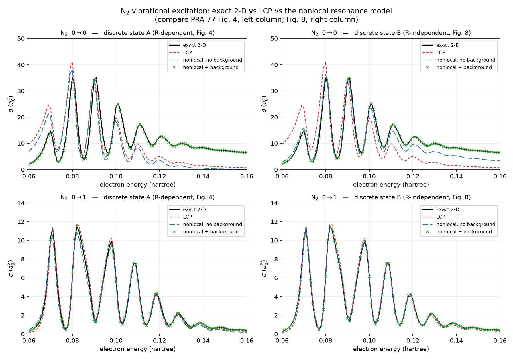
Rows are the transitions (0→0 top, 0→1 bottom); columns are the discrete-state choice —
left is choice A, which is what Fig. 4 plots; right is choice B, which is what Fig. 8
plots. The four curves per panel are the four Fig. 4’s caption defines, in its line
styles, on a linear axis with Fig. 4’s own ticks (0…50 a₀² for 0→0, 0…14 for
0→1) over its own 0.06–0.16 Ha range, so the panels can be laid directly next to the
printed ones. Fig. 8 has no N₂ 0→1 panel, so the bottom-right panel has no published
counterpart — read it against the exact 2-D curve in the same panel.
The line styles match the print; the colours do not. PRA 77 draws the LCP blue short-dashed, the nonlocal-without-background green long-dashed and the +background crosses red; here they are red, blue and green respectively. Pair the curves by dash pattern and marker (and by the legend), not by colour.
101 energies at 0.001 Ha, ten points per boomerang oscillation. Regenerate with
uv run python -m validation.diatomic.ve_nrm_figure
which writes both the PNG and the .npz of all six curves (~14 min; the exact 2-D
sweep dominates). The .npz is gitignored, like every other figure’s data in this
repo — rerun the driver to regenerate it.
Every recorded band in test_ve_nrm.py is measured on an anchor grid, not on every
energy in the window, and two of them are visibly tighter than the dense sweep. The
anchor grid is not the same for both molecules: N₂’s bands are measured on the 11
energies the gate runs, but F₂’s were recorded on the original six-energy sweep and the
gate now runs only the two anchors that bind them (E = 0.02, choice B’s band maximum
and choice A’s worst error; E = 0.04, choice B’s band minimum — the other four sat
strictly inside, so dropping them removed cost and no constraint, and cut the run from
1818 s to 705 s). Widening _ENERGIES["F2"] back to six is a deliberate act.
Choice B widens from _BANDS["N2"] = (0.995, 1.005) to 0.99454–1.00065 —
still inside the 0.7 % headline. Choice A’s 0→1 ratio reaches 1.13260 densely,
outside the recorded _BAND_N2_01 = (0.80, 1.10). Both are grid-sampling differences,
not regressions: a coarse sweep straddles the boomerang peaks where the approximations
are worst. The gate deliberately keeps its 11 energies — the bands are sharp there, and
re-recording on 101 would cost ~14 min inside a test for no gain in detection — so both
dense values are carried as comments next to those two constants. The LCP’s absolute
deviations behave the same way (§6).
10. Cost¶
On the 12-core laptop, one validation.diatomic.ve_nrm.compare call — all six curves,
both choices, both background settings — costs 94.9 s for N₂ at 11 energies (exact
2-D sweep ~63 s, LCP pole walk 4 s, ~2.1–2.6 s per energy per NRM curve) and, for F₂,
705 s at the two anchors the gate runs against 1818 s for the full six-energy
sweep. (An earlier 745.9 s figure for that six-energy sweep is superseded: it did
not reproduce when test_ve_nrm.py re-measured both grids back to back on the same
idle machine, and _ENERGIES records 1818 s as the current cost on this hardware.
That decomposes as ~278 s per energy against ~149 s of fixed setup, so the saving
really does scale with the energy count.) F₂’s cost is dominated by the exact 2-D
sweep at 128,568 unknowns and ~10 GB peak RSS, on top of a 22 s LCP pole walk, 33 s
of grid setup, 2 × 14 s of ingredients and ~10–12 s per energy per NRM curve.
Measured on the figure’s own 101-energy run: 10.5 s of fixed setup plus 8.0 s per
energy for all six curves. As with DA, the exact solve dominates and
sets peak RSS; run the two molecules serially.